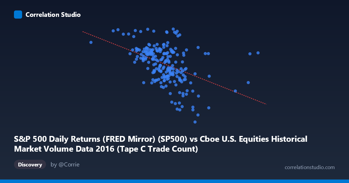
S&P 500 Daily Returns (FRED Mirror) (SP500) vs Cboe U.S. Equities Historical Market Volume Data 2016 (Tape C Trade Count)
- Pearson correlation (r)
- -0.4488
- Spearman correlation
- -0.478
- p-value
- 0
- Sample size (n)
- 224
- 95% confidence interval
- -0.5477 to -0.3376
- Granger causality
- None
- Granger optimal lag
- 1
AI analysis
Analysis: S&P 500 Daily Returns vs. Cboe Tape C Trade Count (2016)
Relationship Overview The scatterplot reveals a moderate negative relationship between S&P 500 daily price levels (X-axis, drawn from the FRED mirror dataset) and Cboe Tape C trade counts (Y-axis). As the S&P 500 index value increases, trade counts on Tape C tend to decline. The linear regression equation (y = −0.0003182x + 2334.68) confirms this inverse slope, suggesting that higher index levels are associated with modestly lower trading activity on this venue. The relationship is visually discernible but far from tight, with considerable scatter throughout the plot.
Correlation Strength and Statistical Significance The Pearson correlation of r = −0.4488 indicates a moderate negative association. However, the coefficient of determination R² = 0.2014 is the more practically meaningful figure: only ~20% of the variance in Tape C trade counts is explained by the S&P 500 level, leaving roughly 80% attributable to other factors. The 95% confidence interval of [−0.5477, −0.3376] is entirely negative, lending confidence to the direction of the relationship, and the p-value of 1.68 × 10⁻¹² confirms this is highly statistically significant — effectively ruling out a chance finding given n = 224 sampled pairs from a population of 2,609 trading-day observations. That said, statistical significance here is partly a function of sample size; practical significance remains limited given the modest R². Critically, Granger causality tests show no significant predictive direction in either direction (X→Y: F = 0.074, p = 0.786; Y→X: F = 0.001, p = 0.979), meaning that neither variable temporally predicts the other at the tested lag, and the correlation should not be interpreted as reflecting any causal or leading-indicator relationship.
Notable Patterns, Clusters, and Outliers The bulk of observations cluster in the X range of roughly 550,000–800,000, corresponding to trade counts between approximately 2,050 and 2,200 — this dense core drives most of the observed correlation. Several notable outliers are visible: a point near X ≈ 1,143,268 (far right) with a trade count near 2,163 sits well outside the main cluster, potentially representing an anomalous high-volume trading day. Similarly, a point near X ≈ 277,976 (far left) with a trade count around 2,213 anchors the lower-X extreme. At the lower end of trade counts (~1,865–1,950), a handful of points appear at mid-to-high X values, suggesting episodic periods of suppressed Tape C activity coinciding with elevated index levels. The spread in Y appears somewhat wider at lower X values, hinting at possible heteroscedasticity.
Confounding Factors and Interpretive Caveats Several important caveats apply. First, the X-axis is labeled as "S&P 500 Daily Returns" but the value range (~278K to ~1.19M) is inconsistent with either the S&P 500 price index (typically 1,800–2,300 in 2016) or return values — this strongly suggests the X variable may actually represent notional trading volume or another market volume metric, and the axis label may be a dataset join artifact, warranting verification. Second, the 2016 timeframe encompasses notable macro events — the February market correction, Brexit (June), and the U.S. election (November) — each of which could independently spike both volume and volatility, acting as confounders. Third, Tape C specifically covers NYSE Arca-listed securities; shifts in market share across venues during 2016 could influence trade counts independently of index levels. Finally, the absence of Granger causality at lag-1 does not preclude relationships at longer lags or non-linear dynamic effects.
Actionable Insights and Further Investigation Given the unexplained 80% of variance, practitioners should explore additional predictors such as VIX (implied volatility), bid-ask spreads, or cross-venue market share data to build a more complete model of Tape C activity. The suspicious X-axis scale should be reconciled and relabeled before drawing any conclusions — if X truly represents a volume metric rather than returns, the economic interpretation changes substantially. It would be worthwhile to test non-linear specifications (e.g., polynomial or piecewise regression) given the visible curvature and heteroscedasticity hints. Extending the Granger causality test to lags 2–10 would provide a more robust picture of any delayed temporal dynamics. Finally, segmenting the data by market regime (low vs. high volatility periods, pre/post-election) may reveal sub-period relationships obscured in the aggregate correlation.
X dataset: Cboe U.S. Equities Historical Market Volume Data 2016
Y dataset: S&P 500 Daily Returns (FRED Mirror)
Part of experiment: Daily - Cboe U.S. Equities Historical Market Volume Data 2016 vs S&P 500 Daily Returns (FRED Mirror)