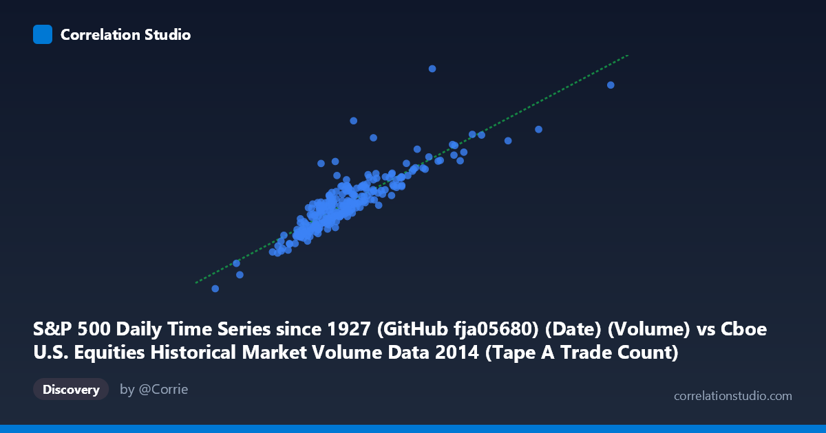
S&P 500 Daily Time Series since 1927 (GitHub fja05680) (Date) (Volume) vs Cboe U.S. Equities Historical Market Volume Data 2014 (Tape A Trade Count)
- Pearson correlation (r)
- 0.876
- Spearman correlation
- 0.8797
- p-value
- 0
- Sample size (n)
- 252
- 95% confidence interval
- 0.8437 to 0.9019
- Granger causality
- None
- Granger optimal lag
- 10
AI analysis
Analysis: S&P 500 Daily Volume vs. Cboe Tape A Trade Count (2014)
Relationship Overview The scatterplot reveals a strong positive linear relationship between S&P 500 daily trading volume and Cboe U.S. Equities Tape A trade count throughout 2014. As daily share volume increases, the number of discrete trades on Tape A rises correspondingly, which is intuitive — higher volume days tend to reflect greater market participation, manifesting simultaneously in both aggregate share counts and individual transaction counts. The linear regression equation (y = 2380.32x + 5.31×10⁸) suggests that for every additional unit of daily volume, Tape A trade count increases by approximately 2,380 trades, with a substantial baseline intercept reflecting a floor of trading activity independent of volume fluctuations.
Correlation Strength and Statistical Significance The correlation is strong and statistically robust: r = 0.876, with an r² of 0.767, meaning approximately 76.7% of the variance in Tape A trade count is explained by daily S&P 500 volume. The 95% confidence interval for r is [0.844, 0.902], a tight band that confirms this is not a chance association, and the p-value is effectively zero across a paired sample of 252 observations drawn from a population of 3,686 trading records. However, the Granger causality analysis tells a more cautious story — neither direction (X→Y nor Y→X) achieves statistical significance (F = 0.849, p = 0.582 and F = 0.805, p = 0.624, respectively, at a 10-period optimal lag). This means that while the two series move together contemporaneously, neither reliably predicts the other in a temporally leading sense. The correlation likely reflects a shared underlying driver rather than a directional causal mechanism.
Notable Patterns, Clusters, and Outliers The bulk of observations cluster tightly in a central region roughly spanning 900,000–1,400,000 in volume and 2.5–4.0 billion in trade count, consistent with typical 2014 trading conditions. However, several notable outliers are visible in the upper-right quadrant: points such as (2,171,498; 5.07B) and (1,834,381; 4.96B) represent unusually high-volume, high-activity sessions that likely correspond to specific market events — index rebalancing dates, macro announcements, or volatility spikes. At the lower-left extreme, the point near (527,319; 1.42B) stands out as a conspicuously low-volume, low-activity session, potentially a holiday-shortened trading day. The dispersion around the regression line widens at higher volume levels, suggesting mild heteroscedasticity — the relationship becomes less precise under extreme market conditions.
Confounding Factors and Interpretive Caveats The most important caveat is that both variables likely respond to the same latent market conditions — volatility regimes, macroeconomic announcements, earnings seasons, and end-of-quarter rebalancing — rather than influencing each other directly. This is precisely what the Granger causality null result implies. Additionally, Tape A specifically covers NYSE-listed securities, while the S&P 500 volume figure aggregates more broadly; compositional differences in what each metric captures could introduce noise and partially suppress the correlation. The single-year (2014) time window is also a limitation — 2014 was a relatively low-volatility year for U.S. equities, and the relationship's structure could differ materially in stress periods like 2008 or 2020. Finally, secular trends in algorithmic trading and market microstructure (e.g., order fragmentation inflating trade counts independently of volume) could confound straightforward interpretation.
Actionable Insights and Further Investigation The strong contemporaneous correlation makes this pairing useful as a cross-validation or anomaly detection tool: extreme divergence between volume and trade count on any given day could signal unusual market microstructure events (e.g., a few very large block trades inflating volume without proportional trade count, or high-frequency activity spiking trade count with minimal share movement). To deepen this analysis, investigators should: (1) extend the time series beyond 2014 to test stability across different volatility regimes; (2) decompose the residuals to identify which specific dates produce the largest deviations and whether those align with known market events; (3) test non-linear specifications given the apparent heteroscedasticity at high volumes; and (4) introduce volatility measures (e.g., VIX) as a covariate to formally test the shared-driver hypothesis implied by the Granger non-causality finding.
X dataset: Cboe U.S. Equities Historical Market Volume Data 2014
Y dataset: S&P 500 Daily Time Series since 1927 (GitHub fja05680) (Date)
Part of experiment: Daily - Cboe U.S. Equities Historical Market Volume Data 2014 vs S&P 500 Daily Time Series since 1927 (GitHub fja05680) (Date)