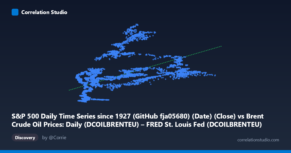
S&P 500 Daily Time Series since 1927 (GitHub fja05680) (Date) (Close) vs Brent Crude Oil Prices: Daily (DCOILBRENTEU) – FRED St. Louis Fed (DCOILBRENTEU)

Pearson correlation (r): 0.5378
Spearman correlation: 0.6915
p-value: 0
Sample size (n): 8140
95% confidence interval: 0.5221 to 0.553
Granger causality: None
Granger optimal lag: 1

AI analysis

Analysis: Brent Crude Oil Price vs. S&P 500

1. What the Visualization Reveals

The scatterplot displays the relationship between daily Brent Crude Oil prices (X-axis, USD per barrel) and S&P 500 closing values (Y-axis) across over three decades of market history (1987–2019). The overall pattern shows a positive but diffuse relationship: as crude oil prices rise, S&P 500 values tend to be higher, but the scatter is substantial and wide. The linear regression line (y = 11.521x + 650.956) captures a modest upward trend, but the cloud of points around it is broad, immediately signaling that oil price alone is a weak predictor of equity market levels. Notably, several distinct clusters are visible, likely reflecting different macroeconomic eras — periods of low oil prices paired with modest equity values (lower-left), and periods of high oil prices coinciding with elevated equity levels (upper-right), though with considerable overlap and exceptions.

2. Strength, Direction, and Statistical Meaning

The Pearson correlation of r = 0.5378 indicates a moderate positive relationship, but the explanatory power is modest: R² = 0.289, meaning only ~28.9% of the variance in S&P 500 values is explained by Brent Crude prices, leaving over 71% attributable to other forces entirely. The 95% confidence interval of [0.5221, 0.5530] is narrow — a function of the large paired sample (n = 8,140) — confirming the estimate is precise, and the p-value of essentially zero confirms this correlation is statistically distinguishable from zero. However, statistical significance should not be conflated with practical significance: a 29% R² in a noisy, multi-driver system like global equities is informative but far from actionable on its own. Critically, the Granger causality results show no significant predictive direction in either direction (X→Y: F = 0.9039, p = 0.342; Y→X: F = 0.8629, p = 0.353), meaning neither variable meaningfully predicts the other's future values at a one-period lag. This is a vital distinction — the correlation is contemporaneous and structural, not a temporal leading indicator.

3. Notable Patterns, Clusters, and Non-Linear Features

Several structural features stand out. There is a dense cluster of points in the lower-left (oil < ~30 USD/bbl, S&P < ~1,000), consistent with the late 1980s and early 1990s market environment. A second, more dispersed cluster occupies the mid-range (oil $40–$80, S&P 1,000–2,500), representing the 2000s commodity boom years. The Spearman ρ exceeding Pearson r is an important diagnostic flag: the relationship is likely non-linear, with a logarithmic or polynomial fit potentially explaining materially more variance than the current linear model. Some notable outliers are visible — high oil prices (~$100+/bbl) paired with relatively modest S&P values, and conversely, modest oil prices with elevated equity readings — consistent with the post-2014 oil price collapse period when equities continued rising. This divergence in the upper-right region is particularly striking and suggests the relationship is regime-dependent.

4. Confounding Factors and Interpretive Caveats

The most important caveat is the shared trend problem: both Brent Crude and the S&P 500 exhibit long-run upward trends over the 1987–2019 period, driven by inflation, economic growth, and USD depreciation. Much of the observed correlation may be spurious co-trending rather than a genuine structural relationship — both variables rising over decades for entirely independent reasons. Additionally, the relationship between oil and equities is context-dependent: rising oil prices driven by demand growth (economic expansion) tend to coincide with rising equities, while supply-shock-driven oil spikes (e.g., Gulf War, 2008) can accompany equity downturns — the opposite dynamic. Sector composition of the S&P 500 also matters, as energy sector weighting has shifted significantly across this period. Finally, the absence of Granger causality at a one-period lag may be lag-specification sensitive; longer lags or different frequencies might yield different results.

5. Actionable Insights and Further Investigation

Given the non-linearity signal, a logarithmic regression (log(X) → Y) or polynomial fit should be tested immediately to determine whether R² improves meaningfully beyond 28.9%. Regime-segmented analysis — separating demand-driven vs. supply-shock oil price environments, or breaking the data into sub-periods (pre/post-2008, pre/post-2014 oil crash) — would likely reveal meaningfully different correlations across eras and resolve the cluster structure observed. Testing Granger causality at multiple lags (2–10 periods, weekly or monthly aggregation) is warranted before concluding there is truly no temporal relationship. For practical investment use, this correlation is insufficient for directional trading signals but may be useful as a macro regime indicator when combined with additional variables (USD index, global PMI, yield curve) in a multivariate framework. Cointegration testing (Engle-Granger or Johansen) would also clarify whether any long-run equilibrium relationship exists between these two series beyond the shared trend.

X dataset: Brent Crude Oil Prices: Daily (DCOILBRENTEU) – FRED St. Louis Fed

Y dataset: S&P 500 Daily Time Series since 1927 (GitHub fja05680) (Date)

Part of experiment: Daily - Brent Crude Oil Prices: Daily (DCOILBRENTEU) – FRED St. Louis Fed vs S&P 500 Daily Time Series since 1927 (GitHub fja05680) (Date)