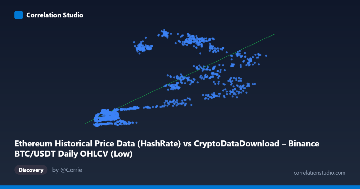
Ethereum Historical Price Data (HashRate) vs CryptoDataDownload – Binance BTC/USDT Daily OHLCV (Low)
- Pearson correlation (r)
- 0.7542
- Spearman correlation
- 0.758
- p-value
- 0
- Sample size (n)
- 1855
- 95% confidence interval
- 0.7338 to 0.7731
- Granger causality
- None
- Granger optimal lag
- 1
AI analysis
Analysis: Ethereum Hash Rate (X) vs. BTC/USDT Low Price (Y)
1. Overview of the Relationship
The scatterplot shows a positive, moderately strong association between the X variable (labeled as Ethereum hash rate, though the values ~2,800–66,000 suggest this may actually represent a price or derived metric rather than raw hash rate) and Y (BTC/USDT daily low price). As X increases from its lower range (~3,000–10,000) toward higher values (~40,000–66,000), Y rises correspondingly from roughly ~100–250 up to 700–1,065. The sample points suggest a generally upward-sloping cloud of data consistent with the fitted linear regression line: y = 0.0131x + 114.83.
2. Strength, Direction, and Statistical Confidence
The correlation coefficient r = 0.754 indicates a strong positive linear relationship, and r² = 0.569 means approximately 57% of the variance in BTC low price is statistically explained by this X variable — a substantial but incomplete share, leaving ~43% of variance driven by other factors. The 95% CI [0.734, 0.773] is tight, and combined with p ≈ 0, this confirms the correlation is highly unlikely to be due to chance, given the large sample (n=1,855). However, correlation strength should not be conflated with causation: the Granger causality tests show no significant predictive direction (X→Y: p=0.266; Y→X: p=0.512). This means neither variable reliably predicts future movements of the other in a time-lagged sense — the relationship appears to be contemporaneous/co-integrated (likely both driven by shared market-wide crypto trends) rather than one causally leading the other.
3. Notable Patterns and Outliers
The data is not uniformly linear — there's evidence of heteroscedasticity: variance in Y increases substantially as X grows. At low X (~3,000–15,000), Y is tightly clustered between ~100–250. At higher X (~20,000–55,000), Y spreads dramatically, ranging from ~270 (e.g., X=26,101, Y=289) to over 1,000 (e.g., X=29,255, Y=1,016; X=35,258, Y=1,008) at similar X levels. This suggests regime-dependent behavior — likely reflecting different market cycles (e.g., 2017–2018 bull run vs. 2020–2021 bull run) where similar X values coincide with very different Y levels depending on the time period. This is a classic sign of non-stationarity in crypto time series, where price levels shift structurally over multi-year periods rather than following a single stable linear relationship.
4. Confounding Factors and Caveats
Several caveats are critical here: - Temporal/trend confounding: Both BTC and ETH-related metrics have grown over the 2017–2022 period alongside overall crypto market adoption, macro liquidity conditions, and speculative cycles. A shared upward trend across unrelated crypto assets can produce spurious correlation even without direct causal linkage. - Metric ambiguity: The X-axis label ("Ethereum Historical Price Data (HashRate)") is inconsistent with typical hash rate magnitudes and value ranges — it may actually be a price-like metric, which would make this a price-price relationship (common and expected to correlate across crypto assets due to shared market sentiment). - Autocorrelation: Both series are daily time series with strong internal autocorrelation, which can inflate apparent correlation strength in simple Pearson calculations, and the Granger results (using only 1 lag) may not fully capture longer-term lead-lag dynamics.
5. Suggested Next Steps
To clarify the true relationship, analysts should: (1) confirm the actual definition/units of the X variable to resolve the hash-rate-vs-price ambiguity; (2) test cointegration (e.g., Engle-Granger) rather than relying solely on levels correlation, given the non-stationary, trending nature of crypto prices; (3) segment the analysis by bull/bear market regimes to check if the r² and slope are stable or regime-dependent, given the heteroscedastic fan pattern observed; and (4) extend Granger tests to multiple lag structures (weekly/monthly) since daily lag-1 may be too short to capture meaningful cross-asset lead-lag effects in crypto markets.
X dataset: CryptoDataDownload – Binance BTC/USDT Daily OHLCV
Y dataset: Ethereum Historical Price Data
Part of experiment: Bitcoin - CryptoDataDownload – Binance BTC/USDT Daily OHLCV vs Ethereum Historical Price Data