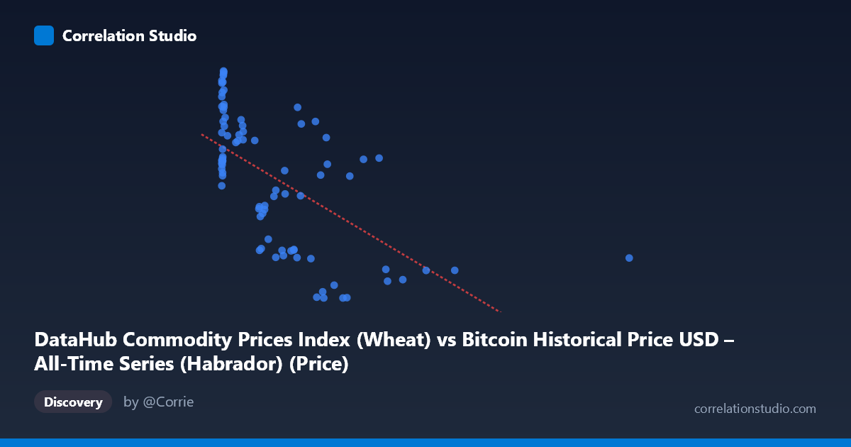
DataHub Commodity Prices Index (Wheat) vs Bitcoin Historical Price USD – All-Time Series (Habrador) (Price)
- Pearson correlation (r)
- -0.6083
- Spearman correlation
- -0.6304
- p-value
- 0
- Sample size (n)
- 83
- 95% confidence interval
- -0.7284 to -0.4519
- Granger causality
- None
- Granger optimal lag
- 10
AI analysis
Analysis: Wheat Price Index vs. Bitcoin Historical Price USD
1. Overview of the Relationship
The scatterplot reveals a moderate negative relationship between the wheat commodity price index (X-axis) and Bitcoin price in USD (Y-axis). Data points cluster heavily in the lower-X range (below ~700), with Y-values spread across roughly 122–320. As X increases beyond ~700, Y-values consistently compress into a narrower lower band (roughly 122–260), producing the visual impression of a downward-sloping trend, though with considerable scatter—especially at low X values.
2. Strength, Direction, and Statistical Confidence
The correlation coefficient (r = -0.608) indicates a moderate negative linear relationship, with r² = 0.370 meaning only 37% of the variance in Bitcoin price is explained by wheat index levels—leaving 63% attributable to other factors. The 95% CI [-0.728, -0.452] is reasonably tight and entirely negative, and the p-value (1.06E-09) is highly significant, giving strong confidence that this negative association is not due to chance in this sample. However, statistical significance should not be conflated with practical predictive power: with r² well below 0.5, wheat prices alone are a weak-to-moderate predictor of Bitcoin price. Critically, the Granger causality tests show no significant predictive direction in either direction (X→Y: p=0.40; Y→X: p=0.19), meaning neither series reliably forecasts the other over time. This suggests the correlation is likely driven by a shared underlying trend or coincidental co-movement over the 2010–2017 period rather than genuine causal influence.
3. Notable Patterns and Outliers
Several structural features stand out: - Clustering at low X (0–50): A dense cluster of points with high Y-values (240–320) sits near X≈0–20, representing early Bitcoin price history when wheat index data may have limited variation—this cluster heavily anchors the regression's left side. - High-X outlier: The point (2452.18, 157.20) is a substantial leverage point, isolated far to the right of the main data cloud, which can disproportionately influence the slope estimate. - Non-linear suggestion: The relationship looks more like two regimes—one with high Y variance at low X, and a compressed, lower Y-band at high X—rather than a strictly linear decline, hinting at a possible threshold or non-linear (e.g., logarithmic) relationship rather than a clean straight-line trend. - Mid-range scatter: Between X=200–800, Y-values vary widely (from ~120 to ~290), showing weak local correlation and suggesting other variables drive Bitcoin price in this range.
4. Confounding Factors and Caveats
This is a classic case where temporal alignment, not causal linkage, likely drives the correlation. Both Bitcoin price and commodity indices were influenced by macroeconomic conditions (USD strength, global liquidity, post-2008 recovery, inflation expectations) over 2010–2017, creating spurious correlation through shared time trends rather than direct interaction. Additionally, n=83 paired samples is a small fraction of the full N=449 population, raising sampling representativeness concerns. The high-leverage outlier at X=2452 and the dense early cluster at X≈0 both distort the linear fit—robustness checks (e.g., removing outliers, log-transforming X) are needed. Finally, Bitcoin's youth as an asset in this period (highly volatile, low liquidity in early years) makes it prone to noise unrelated to commodity markets.
5. Recommendations for Further Investigation
- Detrend both series (e.g., first-differencing or removing time trend) before correlating, to test whether the relationship survives after removing shared temporal drift—this is essential given the null Granger causality result. - Test non-linear/log models: given the clustering pattern, log(X) vs. Y or segmented regression may fit better than a simple linear model. - Exclude/flag outliers (especially X=2452.18) and rerun correlation to assess sensitivity. - Introduce a third variable (e.g., USD index, inflation rate) as a control to check if the wheat-Bitcoin correlation is mediated by a common macro factor. - Conclusion for practical use: Given weak r², lack of Granger causality, and likely confounding by shared macro trends, this correlation should not be used for predictive or trading purposes—it's better understood as a historical co-movement artifact than an exploitable causal relationship.
X dataset: Bitcoin Historical Price USD – All-Time Series (Habrador)
Y dataset: DataHub Commodity Prices Index
Part of experiment: Bitcoin - Bitcoin Historical Price USD – All-Time Series (Habrador) vs DataHub Commodity Prices Index