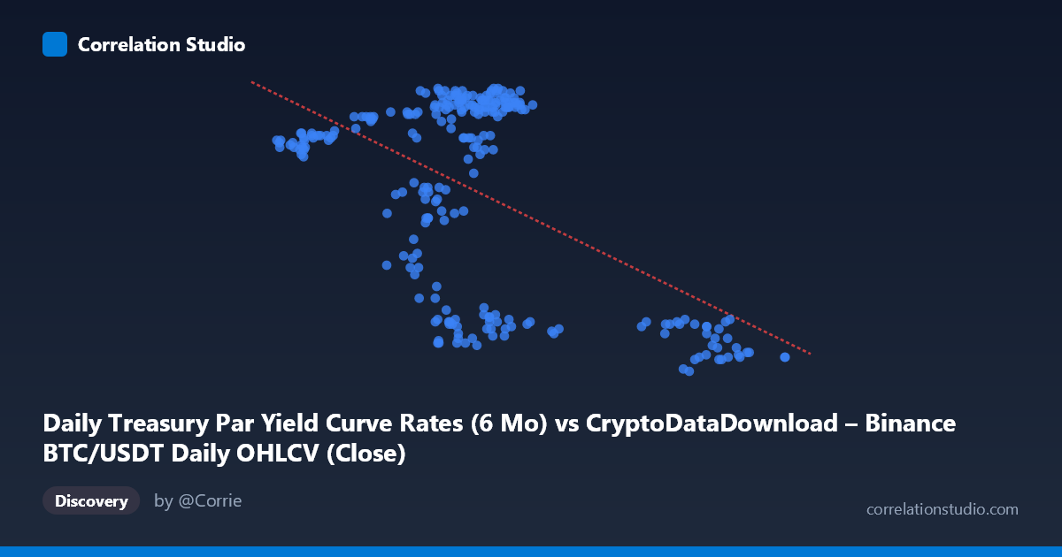
Daily Treasury Par Yield Curve Rates (6 Mo) vs CryptoDataDownload – Binance BTC/USDT Daily OHLCV (Close)

Pearson correlation (r): -0.5451
Spearman correlation: -0.1992
p-value: 0
Sample size (n): 250
95% confidence interval: -0.6267 to -0.4515
Granger causality: None
Granger optimal lag: 1

AI analysis

Analysis of Treasury 6-Month Yield vs. BTC/USDT Close Price

1. Overview of the Relationship

The scatterplot displays a moderate negative relationship between the 6-Month Treasury Par Yield and BTC/USDT closing prices across 250 paired daily observations from 2024. As the Treasury yield axis (X) increases, the corresponding BTC/USDT value (Y) tends to decrease, though the relationship is far from a tight linear band — there is substantial vertical scatter at most X values, indicating considerable unexplained variance.

2. Strength, Direction, and Statistical Confidence

The correlation coefficient of r = -0.5451 indicates a moderate negative linear association. Squaring this, r² = 0.2971, means only about 30% of the variance in one variable is statistically explained by the other — leaving 70% of the variability attributable to other factors, noise, or non-linear dynamics. The 95% confidence interval [-0.6267, -0.4515] is reasonably narrow and does not cross zero, and the p-value ≈ 0 confirms this negative correlation is highly unlikely to be due to chance at this sample size (n=250). However, correlation strength should not be conflated with predictive power: the Granger causality tests show no significant temporal causality in either direction (X→Y: p=0.60; Y→X: p=0.27). This is a critical distinction — the two series move together contemporaneously but neither reliably leads or forecasts the other at a 1-period lag, suggesting the relationship may be coincidental, driven by a shared external factor, or operating on a different time scale than tested.

3. Patterns, Clusters, and Outliers

The data appears to cluster into at least two distinct regimes rather than following a smooth continuous trend. One dense cluster sits around X≈57,000–70,000 with Y values mostly high (5.0–5.44), and a second, sparser cluster appears around X≈87,000–101,000 with consistently low Y values (4.25–4.43). There's also a middle-range grouping (X≈43,000–47,000) with moderately high Y (~5.2). This clustering pattern — rather than a continuous linear decay — suggests the relationship may be driven by discrete time periods or regime shifts (e.g., yield stayed flat for stretches while price moved, or vice versa) rather than a smooth causal mechanism. This kind of "clumping" can artificially inflate a linear correlation coefficient even when the underlying relationship is more like a step function or driven by autocorrelation within each cluster.

4. Confounding Factors and Caveats

Both series are time-ordered financial/economic data over the same calendar year, making them highly susceptible to autocorrelation and spurious correlation — each variable trends over time independent of the other, and any two trending series can show artificial correlation. Since the Granger tests show no lead-lag predictive relationship, a more plausible explanation is that both are being driven by a common macro factor (e.g., Fed policy expectations, risk-on/risk-off sentiment, inflation data, liquidity conditions) rather than one causing the other. Additionally, daily financial data often exhibits volatility clustering and regime dependence that violates the i.i.d. assumptions underlying standard correlation/regression tests, which may affect the validity of the reported p-value and confidence interval.

5. Recommendations for Further Investigation

Given the lack of Granger causality, analysts should avoid treating this as a tradable causal signal and instead: (1) test for cointegration (e.g., Engle-Granger or Johansen tests) since both series may be non-stationary trending series; (2) examine differenced/returns data rather than levels to reduce spurious correlation from shared trends; (3) explore longer lag structures (weekly, monthly) in Granger tests, since macro rate effects on crypto markets may operate with delays beyond 1 day; and (4) investigate a third-variable model incorporating Fed policy announcements, DXY (dollar index), or equity market risk sentiment as potential common drivers explaining both series' movements simultaneously.

X dataset: CryptoDataDownload – Binance BTC/USDT Daily OHLCV

Y dataset: Daily Treasury Par Yield Curve Rates

Part of experiment: Bitcoin - CryptoDataDownload – Binance BTC/USDT Daily OHLCV vs Daily Treasury Par Yield Curve Rates