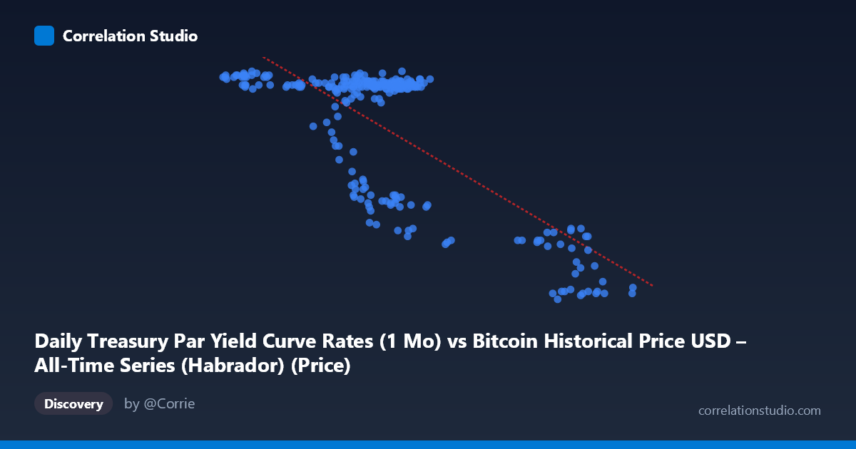
Daily Treasury Par Yield Curve Rates (1 Mo) vs Bitcoin Historical Price USD – All-Time Series (Habrador) (Price)
- Pearson correlation (r)
- -0.7499
- Spearman correlation
- -0.5362
- p-value
- 0
- Sample size (n)
- 250
- 95% confidence interval
- -0.7995 to -0.69
- Granger causality
- None
- Granger optimal lag
- 1
- Time coverage
- 2024-01-02 to 2024-12-31
- Recomputed on refreshed data
- 2026-10-24 (r was -0.7499)
AI analysis
Analysis: Treasury Yield vs. Bitcoin Price Relationship
1. Overall Relationship The scatterplot reveals a clear negative, non-linear relationship between the two variables. At lower X-values (roughly 40,000–70,000), Y clusters tightly in a high band (5.4–5.55), suggesting a plateau or ceiling effect. Once X exceeds ~85,000–90,000, Y drops sharply to a much lower band (4.4–4.7). Rather than a smooth linear decay, the data suggests a threshold/regime-shift pattern: a stable high-Y regime, a sparse transition zone, and a stable low-Y regime, with relatively few points in between.
2. Strength, Direction, and Statistical Confidence The correlation coefficient (r = -0.75) indicates a strong negative linear association, with r² = 0.56 meaning the linear model explains about 56% of the variance in Y — substantial, but leaving ~44% unexplained, consistent with the visible non-linearity described above. The 95% CI [-0.80, -0.69] is tight and does not cross zero, and the p-value ≈ 0 confirms this relationship is highly unlikely to be due to chance at this sample size (n=250). However, the Granger causality tests show no significant predictive direction in either direction (X→Y: p=0.44; Y→X: p=0.78). This is an important caveat: despite the strong contemporaneous correlation, neither series reliably forecasts the other over time — the relationship may be simultaneous, driven by a shared external factor, or structural rather than dynamic/causal.
3. Notable Patterns and Outliers Three sub-clusters stand out: (a) a dense high-Y cluster spanning X ≈ 40,000–70,000 with Y ≈ 5.4–5.55 (the bulk of the data), (b) a secondary mid-tier cluster around X ≈ 58,000–70,000 with Y ≈ 4.7–4.95 (a partial overlap zone, possibly a transitional or seasonal effect), and (c) a distinct high-X/low-Y cluster (X 85,000, Y ≈ 4.4–4.7). The gap between X ≈ 70,000 and 85,000 is sparsely populated, suggesting either a rapid transition or a data/regime discontinuity. This clustering strongly implies a piecewise or step-function relationship rather than a continuous linear one — the linear regression likely understates fit within each regime and overstates it across the transition.
4. Confounding Factors and Caveats Given the axis labels swap oddly in the data description (X reads "Treasury 1-Mo Yield" but values look like BTC prices, and vice versa for Y), there appears to be a column mislabeling in the source metadata — this should be verified before drawing economic conclusions. More substantively, both Treasury yields and Bitcoin prices are driven by common macro factors (Fed policy, inflation expectations, risk-on/risk-off sentiment, liquidity conditions), making it likely that the correlation is confounded by these shared drivers rather than reflecting a direct causal link. Additionally, both series exhibit strong time-trending behavior (non-stationarity), which can inflate correlation coefficients between unrelated trending series — a classic spurious-regression risk that the null Granger causality result reinforces.
5. Recommendations for Further Investigation First, confirm and correct axis/column labeling to ensure the relationship is being interpreted correctly. Second, test for non-stationarity (e.g., ADF tests) and consider differencing or using returns/changes rather than levels to check if the correlation persists — this would help rule out spurious trend-driven correlation. Third, given the visible regime clusters, a piecewise regression, spline model, or regime-switching model would likely fit the data better than a single linear fit and could reveal the X threshold (~75,000–85,000) where the shift occurs. Finally, investigate shared macro covariates (interest rate policy changes, inflation data, liquidity/risk sentiment indices) as potential confounders driving both series simultaneously.
X dataset: Bitcoin Historical Price USD – All-Time Series (Habrador)
Y dataset: Daily Treasury Par Yield Curve Rates
Part of experiment: Bitcoin - Bitcoin Historical Price USD – All-Time Series (Habrador) vs Daily Treasury Par Yield Curve Rates