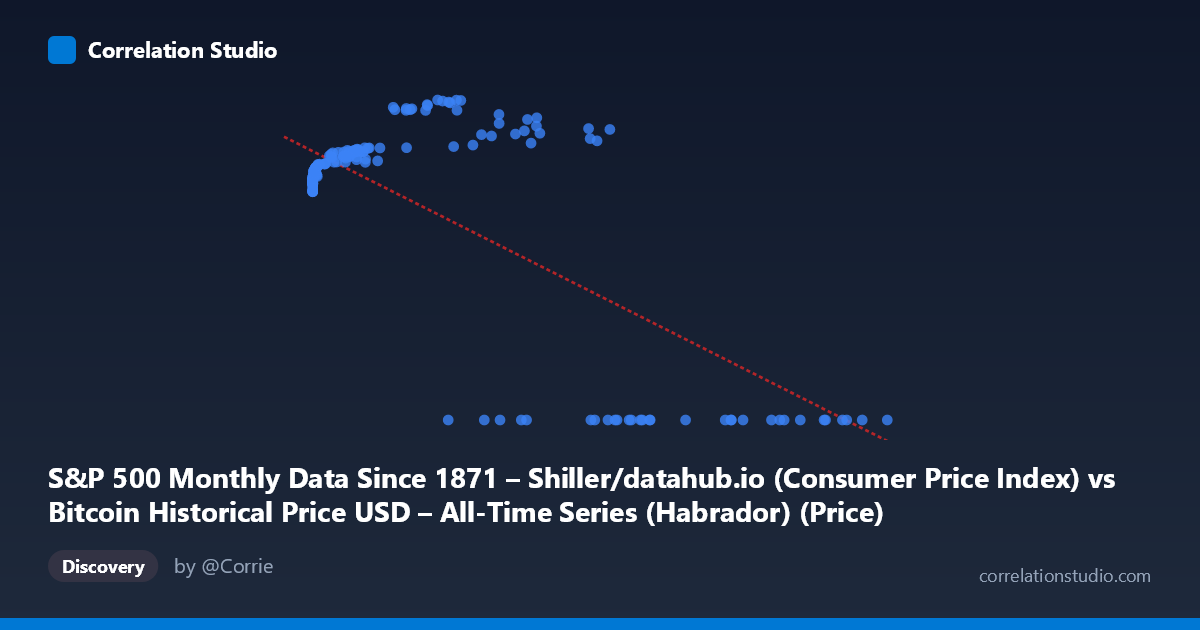
S&P 500 Monthly Data Since 1871 – Shiller/datahub.io (Consumer Price Index) vs Bitcoin Historical Price USD – All-Time Series (Habrador) (Price)
- Pearson correlation (r)
- -0.7354
- Spearman correlation
- 0.1008
- p-value
- 0
- Sample size (n)
- 189
- 95% confidence interval
- -0.7947 to -0.6622
- Granger causality
- Y → X
- Granger optimal lag
- 4
AI analysis
Analysis of Bitcoin Price (X) vs. CPI (Y) Relationship
1. What the Visualization Reveals
Despite the axis labels being somewhat mismatched in the metadata (X appears to actually be Bitcoin price data, Y appears to be CPI values), the scatterplot shows a clear non-linear, negative relationship with a distinctive pattern: Y values cluster tightly around 220-260 for most of the X range, but a substantial subset of points show Y=0.00 exactly, occurring predominantly at high X values (27,000). This bimodal structure—continuous values in one regime and hard zeros in another—suggests the data may represent two different regimes or a data quality/coverage issue (e.g., missing CPI data post-dating available Bitcoin prices, coded as 0).
2. Strength, Direction, and Statistical Uncertainty
The linear correlation (r = -0.735, r² = 0.541) indicates that a linear model explains 54% of the variance in Y from X — a moderate-to-strong relationship, but with nearly half the variance unexplained. The 95% CI [-0.795, -0.662] is reasonably tight and excludes zero, and the p-value of 0 (effectively p < 0.001) confirms this correlation is highly unlikely due to chance alone, especially with n=189 paired observations drawn from a larger population of 1,865. However, the Granger causality results complicate a simple causal story: Y Granger-causes X (F=2.91, p=0.023) is significant, while X→Y is not significant (p=0.056, just above conventional thresholds). This suggests that changes in Y (nominally CPI/inflation-related data) have modest predictive power for future X (Bitcoin price) values at a 4-period lag, but not the reverse — an economically plausible narrative if Y proxies macroeconomic conditions influencing risk-asset pricing.
3. Notable Patterns and Outliers
The most striking feature is the cluster of Y=0.00 values at high X (mostly X 27,000, several exceeding 60,000-118,000) — these are likely artifacts (missing data encoded as zero, or a structural break like Bitcoin prices post-2020 outstripping available matched CPI records) rather than genuine data points. Excluding these, the non-zero Y values show a curved, saturating pattern: Y rises from ~218 near X≈0 up to a peak around 260-306 in the mid-range (X ~7,000-45,000), then the relationship becomes ambiguous. This suggests the true relationship may be logarithmic or power-law rather than linear, which is unsurprising given X's massive scale (0.06 to 118,670) and the log-normal-like distribution typical of asset prices. The linear model's negative slope is likely being driven largely by the zero-cluster at high X values, not by a genuine declining trend in the continuous data.
4. Confounding Factors and Caveats
Several serious caveats apply. First, the column/dataset labeling is confusing and possibly swapped — X is described as CPI data but ranges into hundreds of thousands, consistent with Bitcoin prices, while Y (0-306 range) looks like CPI or an index level, not Bitcoin price. This mismatch should be resolved before drawing economic conclusions. Second, the zero-inflation issue is a major confound: if zeros represent missing/unavailable data rather than true values, they artificially inflate the negative correlation and violate linear regression assumptions (homoscedasticity, linearity). Third, both series are time series with trends (X spans 2010-2026), making them prone to spurious correlation via common trend/non-stationarity — two unrelated upward-trending series will show high correlation even without genuine dependence, and Granger causality itself assumes stationarity, which is unlikely satisfied by raw price levels.
5. Actionable Insights and Next Steps
Before further interpretation: (1) verify and correct axis/column mapping to ensure X and Y correspond to their described variables; (2) investigate and likely exclude or separately model the Y=0 cluster, treating it as missing data rather than a true value, and re-run correlation/regression on the cleaned subset; (3) log-transform X (given its multi-order-of-magnitude range) before fitting, since a log-linear or log-log model will likely fit the continuous data much better than r²=0.54 suggests; (4) difference or detrend both series before Granger testing to guard against spurious causality from shared trends/non-stationarity, and confirm results hold with stationarity-adjusted data (e.g., ADF test, then re-run Granger on returns/differences); and (5) if the CPI–Bitcoin relationship is of genuine interest, supplement with additional macro variables (interest rates, dollar index) to test whether the relationship is direct or mediated by broader monetary conditions.
X dataset: Bitcoin Historical Price USD – All-Time Series (Habrador)
Y dataset: S&P 500 Monthly Data Since 1871 – Shiller/datahub.io
Part of experiment: Bitcoin - Bitcoin Historical Price USD – All-Time Series (Habrador) vs S&P 500 Monthly Data Since 1871 – Shiller/datahub.io