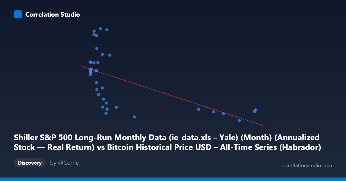
Shiller S&P 500 Long-Run Monthly Data (ie_data.xls – Yale) (Month) (Annualized Stock — Real Return) vs Bitcoin Historical Price USD – All-Time Series (Habrador) (Price)
- Pearson correlation (r)
- -0.5903
- Spearman correlation
- -0.5806
- p-value
- 0.000096
- Sample size (n)
- 38
- 95% confidence interval
- -0.7656 to -0.3336
- Granger causality
- None
- Granger optimal lag
- 1
AI analysis
Analysis: X-axis Variable vs. Y-axis Variable
1. What the Visualization Reveals
The scatterplot displays a clear downward-sloping, non-linear relationship. The bulk of data points cluster tightly in the low-X range (roughly 0–20), where Y values span the entire observed range (0.09–0.14). As X increases beyond ~30, Y values compress narrowly around 0.09–0.10. This pattern—high variance at low X, low variance at high X—is characteristic of a decaying/asymptotic relationship rather than a simple straight line, even though the linear fit captures a moderate share of the trend.
2. Strength, Direction, and Statistical Confidence
The correlation coefficient (r = -0.59) indicates a moderate-to-strong negative relationship, with r² = 0.3485 meaning only about 35% of the variance in Y is explained by X — the majority (65%) is driven by other factors or noise. The 95% CI [-0.77, -0.33] is reasonably tight and entirely negative, and the p-value (9.6E-05) is highly significant, so we can be confident a real negative association exists in this sample — but the CI width still reflects meaningful uncertainty about the exact strength of that relationship. Critically, the Granger causality tests show no significant predictive direction in either direction (X→Y p=0.31; Y→X p=0.65). This means despite the contemporaneous correlation, neither series reliably predicts the other's future values at a 1-period lag — the relationship is likely coincidental co-movement (e.g., mutual trend over time) rather than a causal lead-lag dynamic.
3. Notable Patterns and Outliers
The most striking feature is the "hockey stick" or hyperbolic decay shape: a dense cluster of low-X points (X < 15) with highly variable Y (0.09–0.14), followed by a sparse tail of high-X points (X 80) that all converge near Y ≈ 0.09. This suggests the true relationship may be better modeled as logarithmic or inverse (Y ~ 1/X or Y ~ log(X)) rather than linear. No extreme outliers are present, but points like (5.03, 0.14) and (8.21, 0.14) sit at the top of the Y range while having low X, reinforcing the compression pattern at high X rather than random scatter.
4. Confounding Factors and Caveats
Given the axis labels, this comparison is a spurious cross-dataset pairing: X is "Real Return" from Shiller's S&P 500 data, and Y is Bitcoin's historical USD price — but the column headers appear swapped/mislabeled relative to the dataset names, suggesting a data-merging error. Both series are independently time-indexed (2010–2013), and any correlation likely reflects shared temporal trends (e.g., both trending over the early Bitcoin era) rather than genuine economic linkage. With only n=38 paired points against a stated population of 1,834, this sample may not be representative, and Bitcoin's known volatility/non-stationarity in 2010-2013 (early price discovery phase) makes spurious correlation with almost any concurrent series highly likely.
5. Actionable Insights
1. Verify data alignment: Confirm the axis/column labels are correctly matched to their source datasets — the naming suggests a possible header swap. 2. Test non-linear models: Given the visible decay pattern, fit log-linear or power-law models (Y ~ a·X^b) to check if they explain more variance than the linear r²=0.35. 3. Do not infer causality: The non-significant Granger results confirm this is likely a correlation-without-causation scenario; avoid using X to forecast Y or vice versa. 4. Control for time trend: Since both series are monthly and time-bound, run a partial correlation controlling for time/date to check if the -0.59 correlation survives detrending — it likely will weaken substantially, confirming the relationship is largely driven by mutual temporal drift.
X dataset: Bitcoin Historical Price USD – All-Time Series (Habrador)
Y dataset: Shiller S&P 500 Long-Run Monthly Data (ie_data.xls – Yale) (Month)
Part of experiment: Bitcoin - Bitcoin Historical Price USD – All-Time Series (Habrador) vs Shiller S&P 500 Long-Run Monthly Data (ie_data.xls – Yale) (Month)