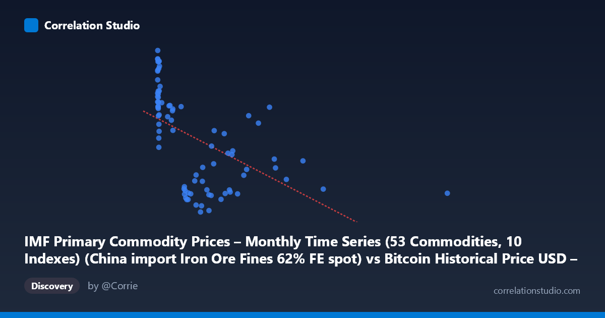
IMF Primary Commodity Prices – Monthly Time Series (53 Commodities, 10 Indexes) (China import Iron Ore Fines 62% FE spot) vs Bitcoin Historical Price USD – All-Time Series (Habrador) (Price)
- Pearson correlation (r)
- -0.5301
- Spearman correlation
- -0.7025
- p-value
- 0
- Sample size (n)
- 83
- 95% confidence interval
- -0.6693 to -0.355
- Granger causality
- None
- Granger optimal lag
- 10
- Time coverage
- 2010-08-01 to 2017-06-01
- Recomputed on refreshed data
- 2026-10-24 (r was -0.5301)
AI analysis
Analysis: Iron Ore Prices vs. Bitcoin Price
1. What the Visualization Reveals
The scatterplot shows a moderate negative relationship between the Iron Ore Fines 62% FE spot price (X-axis) and Bitcoin price (Y-axis). Most data points cluster tightly at low X-values (under ~300), where Bitcoin prices span a wide range (roughly 40–187), while a sparser tail of higher iron ore prices (500–2452) corresponds to consistently lower Bitcoin prices (55–135). This creates a visual impression of decline, but it is heavily shaped by the data's skewed distribution rather than a clean linear trend.
2. Strength, Direction, and Statistical Confidence
The Pearson correlation (r = -0.53, r² = 0.281) indicates a moderate negative association, meaning only about 28% of the variance in Bitcoin price is statistically explained by iron ore prices — leaving 72% unexplained by this relationship alone. The 95% CI [-0.669, -0.355] is reasonably tight and excludes zero, and the p-value (2.55e-07) is highly significant, confirming this correlation is not due to random chance in this sample. However, statistical significance should not be conflated with practical predictive power or causation — r² of 0.28 is a weak-to-moderate fit, unsuitable for reliable forecasting.
Critically, the Granger causality tests show no significant predictive direction in either direction (X→Y: p=0.674; Y→X: p=0.485). This means neither variable's past values help forecast the other's future values over time — despite the contemporaneous correlation, there's no evidence of a lead-lag temporal relationship. This strongly suggests the correlation is likely driven by both series independently trending over the 2010–2017 window (e.g., both influenced by global macro conditions, or simply coincidental co-movement over time) rather than one causing the other.
3. Notable Patterns and Non-linear Features
The data is highly right-skewed on the X-axis (mean 321 vs. stdev 405, max 2452), with most points clustered below X=300 and a long thinning tail extending to 2452. Within the dense low-X cluster, Bitcoin prices vary enormously (40 to 187), showing high scatter and weak local relationship. The high-X tail (X 700) shows a tighter, more consistent negative pattern with lower Y-values. This pattern — dense scatter at low X, sparse but consistent decline at high X — combined with the note that Spearman ρ exceeds Pearson r, suggests a non-linear (possibly logarithmic or power-law) relationship fits better than the linear model, likely because the relationship flattens or curves at extremes rather than declining uniformly.
4. Confounding Factors and Caveats
Several caveats apply: - Time-series confound: Both variables are indexed by time (2010–2017) and likely exhibit trends/autocorrelation independent of each other; correlating two trending time series often produces spurious correlation. - Small effective sample: n=83 paired points from a population of 449 — subsampling may not capture the full dynamic range or short-term volatility. - Bitcoin's extreme volatility in this era (early bull/bear cycles) is driven by idiosyncratic factors (exchange hacks, regulatory news, adoption cycles) unrelated to commodity markets. - Iron ore prices reflect industrial/Chinese demand cycles, a fundamentally different economic driver than crypto speculation. - No mechanism plausibly links iron ore spot prices directly to Bitcoin valuation; any relationship is likely mediated by broader macro factors (USD strength, global risk sentiment, Chinese economic growth) affecting both.
5. Actionable Insights and Further Investigation
- Do not use iron ore prices as a predictive input for Bitcoin price models — the lack of Granger causality confirms no forecasting value despite the contemporaneous correlation. - Test non-linear models (log-log or polynomial regression) given the Spearman/Pearson discrepancy, which may improve fit and better characterize the relationship at extremes. - Detrend both series (e.g., first-differencing or examining returns rather than levels) to check if the correlation persists — this would help distinguish genuine co-movement from shared time-trend artifacts. - Introduce a mediating variable such as a broad risk-asset index, USD index, or Chinese industrial output to test whether it explains the shared variance better than a direct link. - Segment by time period (e.g., pre/post 2013 Bitcoin bubble) to check if the correlation is driven by a specific sub-period rather than being stable across the full range.
X dataset: Bitcoin Historical Price USD – All-Time Series (Habrador)
Y dataset: IMF Primary Commodity Prices – Monthly Time Series (53 Commodities, 10 Indexes)
Part of experiment: Bitcoin - Bitcoin Historical Price USD – All-Time Series (Habrador) vs IMF Primary Commodity Prices – Monthly Time Series (53 Commodities, 10 Indexes)