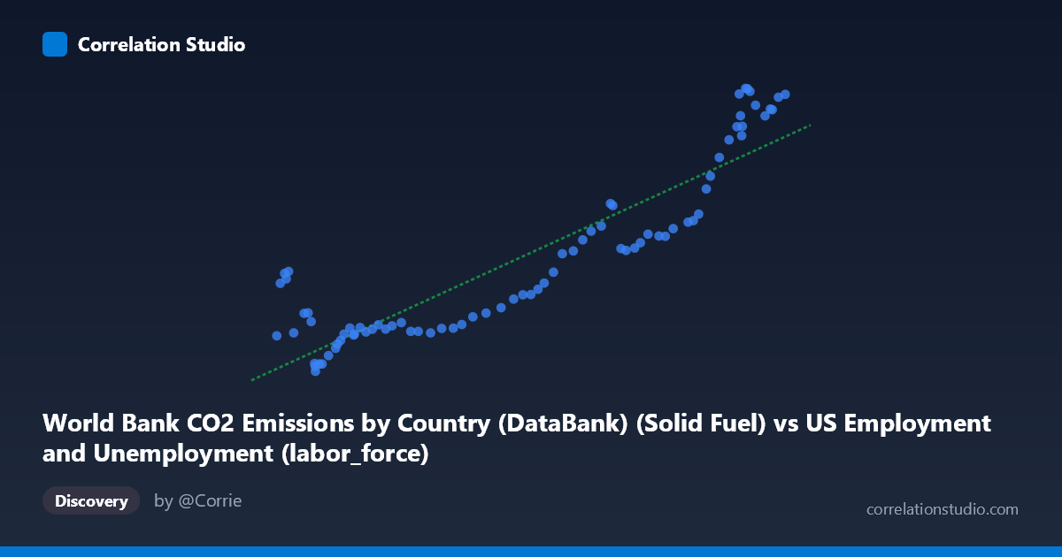
World Bank CO2 Emissions by Country (DataBank) (Solid Fuel) vs US Employment and Unemployment (labor_force)
- Pearson correlation (r)
- 0.9028
- Spearman correlation
- 0.874
- p-value
- 0
- Sample size (n)
- 80
- 95% confidence interval
- 0.8521 to 0.9367
- Granger causality
- None
- Granger optimal lag
- 10
AI analysis
Scatterplot Analysis: Solid Fuel CO2 Emissions vs. US Labor Force
Relationship Overview
The scatterplot reveals a strong positive relationship between World Bank solid fuel CO2 emissions and the US labor force size, with both variables trending upward across the 1941–2020 time coverage. The linear regression equation (y = 0.1616x + 1,050.35) indicates that for every unit increase in solid fuel CO2 emissions, the labor force increases by approximately 0.16 units. Visually, the data points cluster reasonably tightly around the regression line across most of the range, suggesting a consistent co-movement between these two variables over the eight-decade observation window. This relationship almost certainly reflects shared temporal trends — both variables growing alongside postwar economic expansion — rather than any direct mechanistic link.
Correlation Strength and Statistical Inference
The Pearson correlation of r = 0.9028 is statistically strong, and the R² of 0.8150 means that approximately 81.5% of the variance in US labor force size is statistically explained by variation in solid fuel CO2 emissions. The 95% confidence interval [0.8521, 0.9367] is notably narrow given N = 86, and the p-value of essentially zero confirms the result is highly unlikely to be due to random chance. However, statistical significance should not be mistaken for practical or causal significance. The Granger causality tests decisively complicate the narrative: neither direction shows significant predictive causality (X→Y: F = 1.13, p = 0.36; Y→X: F = 1.25, p = 0.29), with an optimal lag of 10 periods. This means that despite the high correlation, knowing past values of one variable does not meaningfully improve forecasts of the other beyond baseline models — a critical caveat for any policy or mechanistic interpretation.
Notable Patterns, Clusters, and Outliers
The scatterplot exhibits several structurally distinct features. At the lower-left end (X roughly 53,000–75,000; Y roughly 9,500–14,000), points cluster more densely and show slightly more scatter relative to the line, suggesting earlier decades when the relationship may have been less stable or the variables were growing at different rates. At the upper-right end (X 150,000; Y 27,000), several points appear to deviate above the regression line, including what appear to be near-ceiling values (e.g., (154,975; 31,153) and (155,389; 31,131)), potentially reflecting recent decades when labor force growth plateaued or accelerated independently of emissions trends. A handful of mid-range points (e.g., (54,630; 16,274) and (55,910; 16,616)) sit noticeably above the regression line, suggesting periods where labor force participation was relatively high despite modest solid fuel emissions — possibly wartime mobilization years in the early 1940s. There are no extreme outliers that would fundamentally distort the regression, but the upper cluster's slight curvature hints at potential non-linearity.
Confounding Factors and Interpretive Caveats
The most significant caveat here is spurious correlation driven by shared time trends. Both the US labor force and global solid fuel CO2 emissions have grown monotonically over most of the 20th century due to entirely independent drivers — population growth, industrialization, and economic development. This is a textbook case where two time-series variables correlate strongly simply because they share a common temporal trajectory, not because they influence each other. Additionally, the dataset pairing is conceptually awkward: "World Bank CO2 Emissions by Country" is a global or multi-country metric being compared to a specifically US labor market variable. Without controlling for global population growth, GDP expansion, or energy transition trends (e.g., coal-to-gas switching), the correlation is largely an artifact of shared secular trends. The failure of Granger causality in both directions further reinforces that no lagged predictive structure underpins the association.
Actionable Insights and Further Investigation
Given these findings, direct policy interpretation (e.g., "reducing emissions will shrink the labor force" or vice versa) would be statistically unwarranted. Instead, meaningful next steps would include: (1) detrending both series (e.g., first-differencing or HP filtering) to remove shared secular trends and re-examining whether any residual correlation persists; (2) decomposing CO2 emissions by country to isolate US-specific solid fuel emissions, which would create a more conceptually coherent pairing with US labor data; (3) testing for structural breaks around key economic events (Great Depression aftermath, 1970s oil shocks, 2008 financial crisis, COVID-19) that may explain the above-line clusters; and (4) introducing control variables such as US GDP, total energy consumption, and working-age population to conduct a proper multivariate analysis. The high R² is more a reflection of the richness of long-run time-series co-movement than evidence of any actionable relationship between emissions and employment.
X dataset: US Employment and Unemployment
Y dataset: World Bank CO2 Emissions by Country (DataBank)
Part of experiment: Yearly - US Employment and Unemployment vs World Bank CO2 Emissions by Country (DataBank)