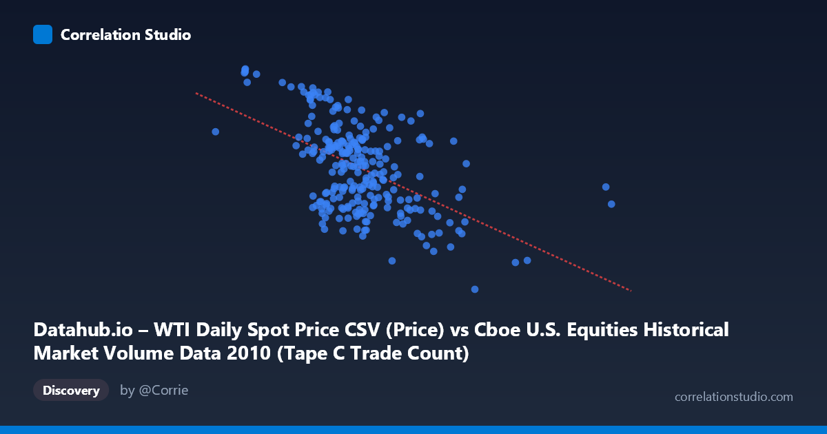
Datahub.io – WTI Daily Spot Price CSV (Price) vs Cboe U.S. Equities Historical Market Volume Data 2010 (Tape C Trade Count)
- Pearson correlation (r)
- -0.5219
- Spearman correlation
- -0.4645
- p-value
- 0
- Sample size (n)
- 252
- 95% confidence interval
- -0.6064 to -0.4258
- Granger causality
- None
- Granger optimal lag
- 1
AI analysis
Analysis: WTI Oil Price vs. Cboe Tape C Trade Count (2010)
Relationship Overview The scatterplot reveals a moderate negative relationship between U.S. equity market trading volume (specifically Tape C trade count, used as the X-axis) and WTI crude oil spot prices (Y-axis) across 252 trading days in 2010. As equity market trade counts increase, oil prices tend to decline, and the linear regression equation (y = -1.807×10⁻⁵x + 90.60) quantifies this downward slope. The relationship is visually apparent but with considerable scatter, suggesting that while a trend exists, many data points deviate substantially from the regression line.
Correlation Strength and Statistical Framing The Pearson correlation of r = -0.5219 indicates a moderate negative association. However, the r² of 0.2724 means that only 27.2% of the variance in WTI oil prices is explained by Tape C trade counts — leaving nearly 73% of price variation unexplained by this variable alone. The 95% confidence interval of [-0.6064, -0.4258] is entirely negative and reasonably narrow given the sample size (n=252), and the p-value of effectively 0 confirms the correlation is statistically significant and unlikely to be a chance finding. That said, statistical significance here is partly a function of the large population context (N=3,302), and practical significance remains modest given the limited explained variance. Crucially, the Granger causality results are non-significant in both directions (X→Y: F=0.72, p=0.397; Y→X: F=3.79, p=0.053), meaning neither variable meaningfully predicts the other temporally with a one-period lag. The Y→X direction approaches but does not cross the conventional significance threshold, hinting weakly that oil prices may have some marginal lagged influence on trading activity, but this should not be overstated.
Notable Patterns, Clusters, and Outliers The data cloud shows a discernible downward trend but with substantial vertical spread at any given X value, particularly in the 450,000–700,000 trade count range where the bulk of observations cluster. Several notable outliers are visible: the point near (1,379,287, 75.10) represents an extreme high-volume trading day far removed from the main cluster, yet its oil price is unremarkable, weakening the trend. Similarly, points near (963,255, 64.78) and (1,086,790, 68.03) show high trade counts paired with low oil prices, consistent with the negative trend. Conversely, low trade-count days (e.g., ~298,000–490,000) tend to cluster at higher oil prices (85–91), anchoring the negative slope. There is also some suggestion of a non-linear or heteroscedastic pattern, with greater spread in Y at moderate X values and tighter clustering at the extremes.
Confounding Factors and Caveats Several important caveats apply. First, both variables are time-series data spanning 2010, meaning the observed correlation may be partly driven by shared temporal trends rather than a direct functional relationship — for instance, oil prices rose broadly in late 2010 while market volumes may have followed independent seasonal or structural patterns. Second, the axis assignments appear inverted from what the column labels suggest (the dataset descriptions indicate X is price and Y is trade count, but the regression slope and ranges suggest otherwise), which warrants verification before drawing directional conclusions. Third, market microstructure factors — including algorithmic trading activity, economic news events, and Federal Reserve policy in the post-crisis environment — likely influenced both variables simultaneously, acting as common drivers. Finally, Tape C specifically covers NYSE Arca-listed securities, which may skew the sample toward ETF and technology trading rather than energy-sector equities.
Actionable Insights and Further Investigation Given the moderate but incomplete correlation and absent Granger causality, this relationship should not be used for predictive modeling without further refinement. Recommended next steps include: (1) controlling for time trends by detrending both series or using first-differences to isolate day-to-day changes rather than levels; (2) extending Granger analysis to longer lags (2–5 periods) to check whether the near-significant Y→X result strengthens; (3) comparing Tape C specifically to energy-sector volume to test whether the relationship is sector-driven; and (4) incorporating additional variables such as VIX (volatility index), USD index, or macroeconomic releases that co-move with both oil prices and equity trading activity. The 2010 timeframe also coincided with post-financial-crisis recovery dynamics, so replicating this analysis across multiple years would help assess whether this correlation is structurally persistent or period-specific.
X dataset: Cboe U.S. Equities Historical Market Volume Data 2010
Y dataset: Datahub.io – WTI Daily Spot Price CSV
Part of experiment: Daily - Cboe U.S. Equities Historical Market Volume Data 2010 vs Datahub.io – WTI Daily Spot Price CSV