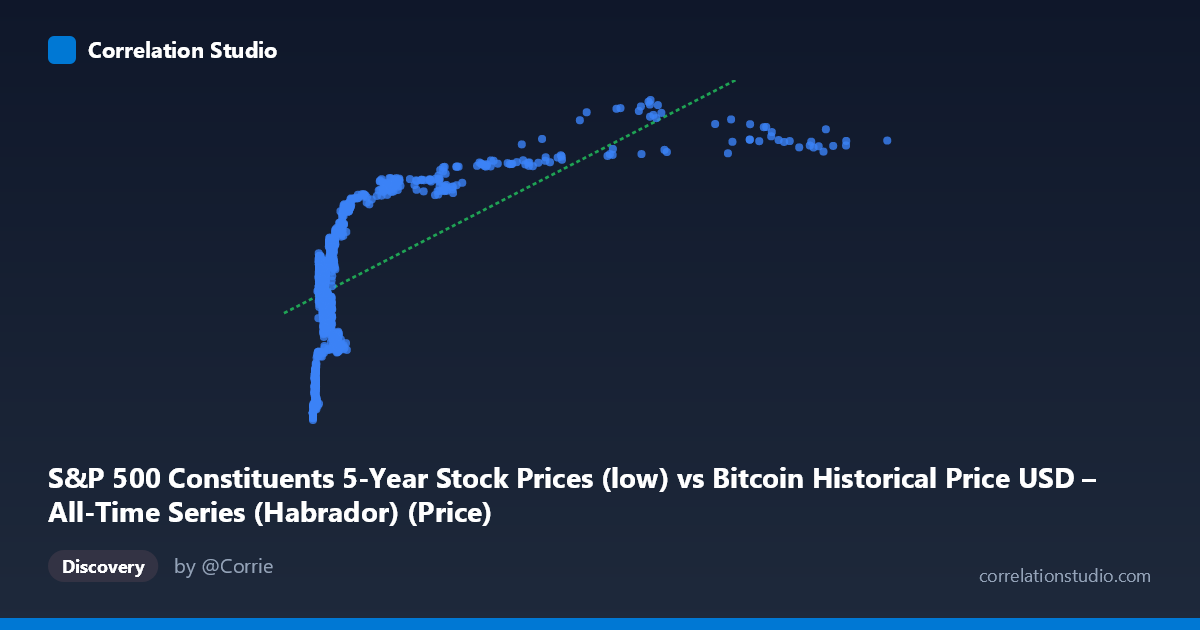
S&P 500 Constituents 5-Year Stock Prices (low) vs Bitcoin Historical Price USD – All-Time Series (Habrador) (Price)
- Pearson correlation (r)
- 0.6348
- Spearman correlation
- 0.7169
- p-value
- 0
- Sample size (n)
- 1259
- 95% confidence interval
- 0.6006 to 0.6667
- Granger causality
- X → Y
- Granger optimal lag
- 1
- Time coverage
- 2013-02-08 to 2018-02-07
- Recomputed on refreshed data
- 2026-10-24 (r was 0.6348)
AI analysis
Analysis: Bitcoin Price vs. S&P 500 Constituent Prices
1. What the Visualization Reveals
The scatterplot shows a positive, non-linear relationship between X (a proxy value labeled as S&P 500-related but ranging into the tens of thousands, consistent with Bitcoin price behavior) and Y (ranging ~57-114, consistent with individual stock price levels). The data shows a clear logarithmic or saturating curve shape: Y rises steeply as X increases from near-zero to about 1,000-2,000, then the rate of increase flattens substantially as X continues to climb toward 10,000+. This is a classic diminishing-returns pattern rather than a straight line, even though the linear fit captures a moderate share of the relationship.
2. Strength, Direction, and Uncertainty
The linear correlation (r = 0.635, R² = 0.403) indicates a moderate-to-strong positive relationship, with about 40% of the variance in Y explained by X — meaning 60% of Y's variance is driven by other factors not captured in this simple relationship. The 95% CI [0.601, 0.667] is tight and does not cross zero, and the p-value of ~0 confirms this correlation is highly statistically significant and not due to chance, especially given the large sample (n=1,259). However, statistical significance here reflects the strength of the pattern, not necessarily a causal mechanism. The Granger causality test adds a temporal dimension: X→Y is significant (F=4.77, p=0.029) while Y→X is not (p=0.652), suggesting X's past values have modest predictive power for future Y values, but not vice versa — though the effect size (F≈4.8) is modest, so this should be treated as suggestive rather than conclusive evidence of true causality.
3. Notable Patterns and Outliers
The most striking feature is the curve's shape: dense clustering of points at low X values (roughly 100-2,000) where Y still varies substantially (60-95), followed by a sparser, more gradual climb at high X values (7,000-19,000) where Y plateaus near 100-113. This suggests a log-linear relationship (Y ~ log(X)) would likely fit better than the stated linear model. There's also a visible "gap" in the X range between roughly 2,500 and 6,900 with few sample points, which may affect the reliability of the fit in that region. No extreme outliers are apparent; the relationship appears consistent across the range, just non-linear.
4. Confounding Factors and Caveats
The variable labels are unusual and likely mismatched or mislabeled in the metadata — X is described as "S&P 500 Constituents" but its range (22 to 18,960) and description reference Bitcoin, while Y is labeled "Bitcoin Historical Price" but its range (57-114) looks like a typical stock price. This strongly suggests a column-swap or labeling error in the source data, which should be resolved before drawing economic conclusions. Additionally, both series are time series covering 2013-2018, a period when Bitcoin experienced massive appreciation and broad equity markets also trended upward — meaning shared macro trends (bull market conditions, monetary policy, risk appetite) could easily produce spurious correlation via mutual time-trending rather than genuine interdependence. Time-series data like this often violates the independence assumptions behind standard correlation/significance tests unless detrended.
5. Suggested Next Steps
First, verify and correct the axis/column labeling to ensure the relationship being tested is the one intended. Second, since both series are likely non-stationary trending time series, apply differencing or log-returns transformation and re-run correlation and Granger causality tests to check whether the relationship holds after removing shared trend effects — this is critical since spurious correlations are common with trending financial time series. Third, fit a log-linear or polynomial model given the visible curvature, which should improve explained variance beyond the current 40%. Finally, given the weak-but-significant Granger result, consider testing additional lags and out-of-sample forecasting performance before treating X as a meaningful leading indicator for Y in any practical/trading context.
X dataset: Bitcoin Historical Price USD – All-Time Series (Habrador)
Y dataset: S&P 500 Constituents 5-Year Stock Prices
Part of experiment: Bitcoin - Bitcoin Historical Price USD – All-Time Series (Habrador) vs S&P 500 Constituents 5-Year Stock Prices