WTI Crude Oil Prices: Daily (DCOILWTICO) – FRED St. Louis Fed (Daily) (DCOILWTICO) vs Cboe U.S. Equities Historical Market Volume Data 2009 (Tape B Trade Count)
- Pearson correlation (r)
- -0.7646
- Spearman correlation
- -0.7395
- p-value
- 0
- Sample size (n)
- 252
- 95% confidence interval
- -0.8115 to -0.7079
- Granger causality
- None
- Granger optimal lag
- 1
AI analysis
Scatterplot Analysis: WTI Crude Oil Prices vs. Cboe Tape B Trade Count (2009)
Relationship Overview
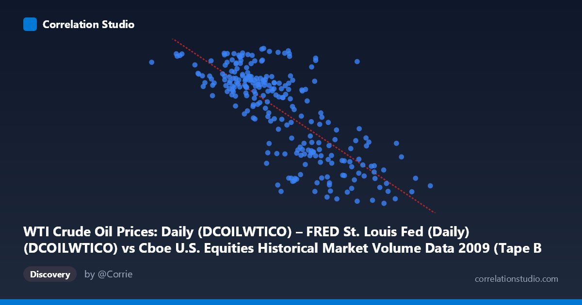
The scatterplot reveals a clear negative relationship between WTI crude oil prices (X-axis, measured in USD per barrel) and Cboe Tape B trade counts (Y-axis) across 252 trading days in 2009. As oil prices rise, trade counts tend to decline, and conversely, lower oil prices are associated with higher trading activity. The linear regression equation (y = -8.206×10⁻⁵x + 94.93) quantifies this inverse slope, suggesting that for every $1,000 increase in the oil price index units used here, trade counts decrease by approximately 0.082 units. The pattern is visually coherent — higher-X observations cluster toward lower Y values, while lower-X points scatter toward higher Y values — though with meaningful dispersion around the trend line.
Correlation Strength, Direction, and Statistical Framing
The Pearson correlation of r = -0.765 indicates a strong negative association, and the R² of 0.585 means that roughly 58.5% of the variance in Tape B trade counts is statistically explained by variation in WTI oil prices — a substantial but incomplete explanation, with ~41.5% of variance attributable to other factors. The 95% confidence interval for r of [-0.812, -0.708] is relatively tight and lies entirely in negative territory, confirming the direction and magnitude of the relationship with high confidence. The p-value of effectively zero (given N = 3,232) makes it virtually certain this correlation is not a statistical artifact. However, the Granger causality tests tell a more cautious story: neither direction (X→Y: F = 0.062, p = 0.804; Y→X: F = 2.312, p = 0.130) achieves significance at conventional thresholds, meaning that past oil prices do not significantly predict future trade counts, and vice versa. This suggests the two variables move together contemporaneously — likely driven by shared underlying forces — rather than one causing the other in a temporally sequential sense.
Notable Patterns, Clusters, and Outliers
Several features stand out on the scatterplot. There is a notable cluster of high trade-count observations (Y 70) concentrated in the lower-to-middle X range (roughly $80,000–$400,000 range units), consistent with the early-2009 period when oil prices were depressed following the 2008 financial crisis and equity market volatility was elevated. Conversely, a cluster of low trade counts (Y < 45) appears at higher X values, corresponding to later-2009 periods as oil prices recovered. A few potential outliers are visible: the point near (81,703, 76.83) sits at the extreme low end of X with a high Y value, and the point near (766,764, 39.35) sits at the extreme high end of X with a notably low Y — both are consistent with the overall trend but anchor the regression line at its extremes. The point cluster around X ≈ 400,000–500,000 shows considerable vertical scatter (Y ranging from ~37 to ~80), suggesting the relationship weakens or becomes noisier in the mid-range of oil prices, possibly indicating a non-linear or threshold dynamic worth investigating.
Confounding Factors and Interpretive Caveats
The most critical caveat is that 2009 was a structurally unique year: it encompassed the tail end of the global financial crisis, a historic market bottom in March, and a sharp recovery through year-end. Both oil prices and equity trading volumes were simultaneously driven by macro risk sentiment, credit conditions, and investor behavior — meaning the observed correlation likely reflects a common response to underlying economic conditions rather than any direct causal link between oil prices and trade counts. The label/axis mismatch in the metadata (X-axis description refers to crude oil, but the dataset attribution appears swapped) warrants careful verification of which series is truly being plotted on which axis. Additionally, Tape B specifically covers NYSE American (formerly AMEX) and regional exchange listings, so these trade counts may reflect sector-specific dynamics (e.g., energy equities, smaller-cap stocks) that happen to correlate with oil prices more strongly than broader market indices would. The absence of Granger causality at lag-1 may also reflect that a longer lag structure or intraday data would be needed to detect any meaningful predictive signal.
Actionable Insights and Further Investigation
Given the strong contemporaneous correlation but absent temporal predictability, analysts should focus on identifying the shared driver — most likely a macro risk-on/risk-off regime variable such as the VIX, credit spreads, or broader market volume — that moves both series simultaneously. A multiple regression framework incorporating macro controls (e.g., S&P 500 returns, VIX, USD index) would help disentangle how much of the oil-trade count correlation survives after accounting for these confounders. Testing longer Granger causality lags (5, 10, or 22 trading days) could reveal whether monthly-horizon predictability exists even if daily lag-1 does not. It would also be valuable to decompose the 2009 data into pre- and post-March sub-periods to test whether the correlation is stable across market regimes or driven primarily by the crisis-to-recovery transition. Finally, replicating this analysis across multiple years would determine whether this relationship is a persistent structural feature or an artifact of the extraordinary 2009 market environment.
X dataset: Cboe U.S. Equities Historical Market Volume Data 2009
Y dataset: WTI Crude Oil Prices: Daily (DCOILWTICO) – FRED St. Louis Fed (Daily)
Part of experiment: Daily - Cboe U.S. Equities Historical Market Volume Data 2009 vs WTI Crude Oil Prices: Daily (DCOILWTICO) – FRED St. Louis Fed (Daily)