S&P 500 Daily Time Series since 1927 (GitHub fja05680) (Date) (Volume) vs Brent Crude Oil Prices: Daily (DCOILBRENTEU) – FRED St. Louis Fed (DCOILBRENTEU)
- Pearson correlation (r)
- 0.759
- Spearman correlation
- 0.8254
- p-value
- 0
- Sample size (n)
- 8140
- 95% confidence interval
- 0.7497 to 0.7681
- Granger causality
- None
- Granger optimal lag
- 10
AI analysis
S&P 500 Trading Volume vs. Brent Crude Oil Price: Correlation Analysis
1. Overall Relationship Revealed
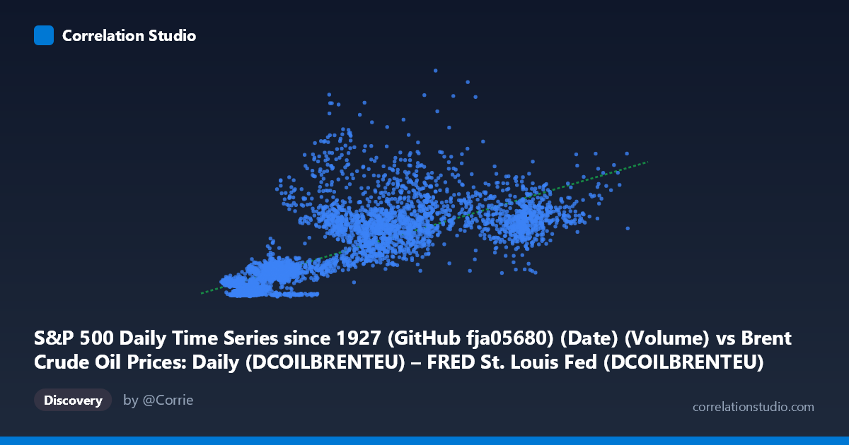
The scatterplot reveals a positive relationship between S&P 500 daily trading volume and Brent crude oil prices, spanning over three decades (1987–2019). As trading volume increases, oil prices tend to rise, with the linear regression equation y = 4.15×10⁷x + 1.08×10⁸ suggesting that each additional unit of volume is associated with a meaningful upward shift in oil price. However, the scatter around this trend line is considerable, indicating that while a broad directional relationship exists, the fit is far from deterministic. The data cloud shows a wide fan-like dispersion, particularly at higher volume levels, hinting at heteroscedasticity — variance in oil prices grows as volume increases.
2. Correlation Strength, Direction, and Causality
The Pearson correlation of r = 0.759 indicates a moderately strong positive association, but the explanatory power deserves careful framing. The R² of 0.576 means that only ~57.6% of the variance in Brent crude prices is explained by S&P 500 trading volume — leaving roughly 42% attributable to other factors entirely. The 95% confidence interval [0.750, 0.768] is notably narrow given the large paired sample (n = 8,140), reflecting high statistical precision rather than a particularly tight real-world relationship. The p-value of ~0 confirms the correlation is statistically indistinguishable from chance only under extraordinary skepticism, but statistical significance here must not be conflated with practical or causal significance. Most critically, the Granger causality tests fail in both directions (X→Y: F = 0.837, p = 0.593; Y→X: F = 0.586, p = 0.827), meaning that neither variable temporally predicts the other at the optimal 10-period lag. This is a crucial finding: despite the moderate correlation, there is no evidence that volume movements lead oil price movements or vice versa.
3. Notable Patterns, Clusters, and Outliers
Several structural features stand out in the data. There is a dense cluster at lower volume and lower oil price values (roughly X < 30, Y < 1B), consistent with earlier years in the sample when both equity market activity and oil prices were lower. A second, more dispersed cluster emerges in the mid-to-high volume range (X: 60–80), with oil prices spanning a wide range from ~2.5B to over 6.5B, suggesting that high-volume trading days are not reliably associated with any particular oil price level. Several apparent outliers are visible — notably the point near (68.66, 6,454,270,000), which sits well above the regression line, and points at high X values (100) such as (109.17, 3,765,770,000) that fall below the trend, suggesting diminishing or inconsistent association at extreme volumes. The vertical spread at any given X value is substantial, reinforcing the heteroscedastic pattern.
4. Confounding Factors and Interpretation Caveats
This correlation almost certainly reflects shared long-run trends rather than a direct economic mechanism. Both S&P 500 trading volume and oil prices have structurally increased over the 1987–2019 period due to independent forces: the secular rise of electronic and algorithmic trading inflating volume, and global demand growth, geopolitical supply shocks, and OPEC dynamics driving oil prices. This creates a classic spurious correlation driven by mutual trending over time — a well-known econometric hazard. The failed Granger causality tests strongly support this interpretation. Additionally, volatility regimes (e.g., the 2008 financial crisis, 2014–2016 oil price collapse) would simultaneously spike trading volume and crash oil prices or vice versa, potentially creating local counter-correlations masked in aggregate statistics. The axis label metadata also appears partially swapped in description, which warrants verification of the variable alignment before drawing firm conclusions.
5. Actionable Insights and Further Investigation
Given the absence of Granger causality, practitioners should avoid using S&P 500 volume as a predictive signal for oil prices (or vice versa) in trading or risk models. A more productive analytical path would involve detrending both series (e.g., via differencing or percentage changes) before re-examining correlation, which would likely substantially reduce r² and reveal the true short-run relationship. It would be valuable to segment the analysis by time period (pre/post 2000, pre/post 2008 crisis) to test whether the correlation is stable or regime-dependent. Incorporating confounding variables such as GDP growth, dollar index movements, or volatility indices (VIX) in a multivariate framework would help isolate whether any genuine information linkage exists. Finally, testing alternative lag structures beyond 10 periods — perhaps at monthly or quarterly aggregation — might surface slower-moving relationships that the daily Granger test misses.
X dataset: Brent Crude Oil Prices: Daily (DCOILBRENTEU) – FRED St. Louis Fed
Y dataset: S&P 500 Daily Time Series since 1927 (GitHub fja05680) (Date)
Part of experiment: Daily - Brent Crude Oil Prices: Daily (DCOILBRENTEU) – FRED St. Louis Fed vs S&P 500 Daily Time Series since 1927 (GitHub fja05680) (Date)