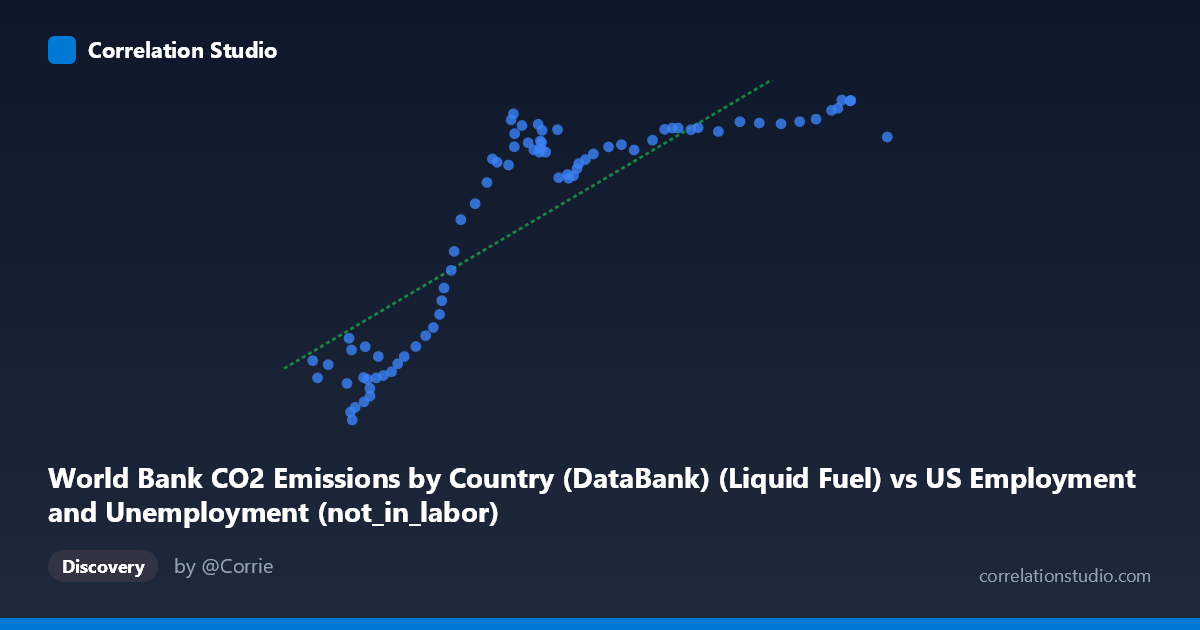
World Bank CO2 Emissions by Country (DataBank) (Liquid Fuel) vs US Employment and Unemployment (not_in_labor)
- Pearson correlation (r)
- 0.831
- Spearman correlation
- 0.8752
- p-value
- 0
- Sample size (n)
- 80
- 95% confidence interval
- 0.7478 to 0.8885
- Granger causality
- None
- Granger optimal lag
- 10
- Time coverage
- 1941-01-01 to 2020-01-01
AI analysis
Scatterplot Analysis: Liquid Fuel CO2 Emissions vs. US Labor Force Non-Participation
1. Overall Relationship
The scatterplot reveals a positive, moderately strong relationship between World Bank liquid fuel CO2 emissions and the number of Americans not in the labor force. As liquid fuel CO2 emissions increase (ranging from ~38,590 to ~99,587 units), the "not in labor force" count rises correspondingly from roughly 2,497 to 13,602. However, the relationship is clearly non-linear — the data exhibits a pronounced S-curve or saturation pattern, with steep gains in Y at lower X values (roughly 38,000–65,000), followed by a plateau where Y flattens considerably despite X continuing to climb toward 100,000. This non-linearity is an important structural feature that the fitted linear regression (y = 0.1935x − 2,595.53) only partially captures.
2. Correlation Strength, Explained Variance, and Causality
The Pearson correlation of r = 0.831 indicates a strong positive association, and R² = 0.691 means the linear model explains approximately 69% of the variance in non-labor-force participation — a substantial but imperfect fit, consistent with the visible non-linearity. The 95% confidence interval [0.748, 0.889] is relatively tight and excludes zero entirely, and the p-value ≈ 0 confirms this is highly statistically significant with N = 80 paired observations across 1941–2020. That said, Granger causality tests find no significant temporal predictive direction in either direction (X→Y: F = 0.94, p = 0.51; Y→X: F = 1.23, p = 0.30), even at the optimal lag of 10 periods. This is a critical finding — despite a strong contemporaneous correlation, neither variable reliably predicts the other forward in time, strongly cautioning against any causal interpretation.
3. Notable Patterns, Clusters, and Outliers
Three visually distinct regions emerge in the scatterplot: - Lower cluster (X ≈ 38,000–55,000; Y ≈ 2,500–7,500): Points are tightly grouped with steep positive slope — small increases in X correspond to large jumps in Y. This likely reflects mid-20th century data where both variables were growing rapidly together. - Transition zone (X ≈ 55,000–68,000; Y ≈ 9,500–12,500): A rapid transition region where Y rises sharply and variability increases noticeably. - Upper plateau (X ≈ 68,000–99,587; Y ≈ 11,000–13,600): Points cluster densely with a near-flat slope — Y saturates around 12,000–13,600 regardless of X continuing to grow. The point at (99,587; 12,317) and several near (94,000–95,000; ~13,300–13,600) appear near the ceiling of Y but are not extreme outliers per se. The point at (42,787; 2,497) represents the absolute minimum on both axes and sits somewhat isolated, warranting verification.
4. Confounding Factors and Caveats
Several important caveats apply. First, this is almost certainly a spurious correlation driven by shared temporal trends — both liquid fuel CO2 emissions and US non-labor-force participation increased substantially across 1941–2020 due to independent structural forces (industrialization, population aging, demographic shifts). Second, the dataset labeling appears cross-joined: the X-axis draws from a US Employment dataset while Y draws from a World Bank CO2 dataset, suggesting these columns may have been matched by year rather than by any direct mechanism. Third, the saturation pattern in the upper range suggests the relationship breaks down entirely at higher emission levels — a linear model is inappropriate here and is visibly overfitting the lower-X region while underfitting the plateau. Finally, the 10-period Granger lag (~10 years) may be too long or methodologically mismatched for these annual series.
5. Actionable Insights and Further Investigation
Given the non-linear shape, a logistic or piecewise regression would likely yield a meaningfully better fit than the current linear model and should be tested. Researchers should detrend both series (e.g., by differencing or controlling for year/population) before drawing any conclusions — once shared time-trend is removed, the residual correlation may diminish substantially or disappear. It would be valuable to investigate the breakpoint around X ≈ 65,000–68,000 (likely corresponding to a specific decade transition) to understand what structural change caused Y to plateau. Cross-validation with population-normalized metrics (per-capita emissions, labor force participation rate rather than raw counts) would provide a more meaningful economic comparison. Finally, the apparent dataset cross-join should be explicitly documented and justified — if this correlation exists purely through shared annual timestamps, it represents a textbook example of spurious temporal correlation requiring careful methodological disclosure.
X dataset: US Employment and Unemployment
Y dataset: World Bank CO2 Emissions by Country (DataBank)
Part of experiment: Yearly - US Employment and Unemployment vs World Bank CO2 Emissions by Country (DataBank)