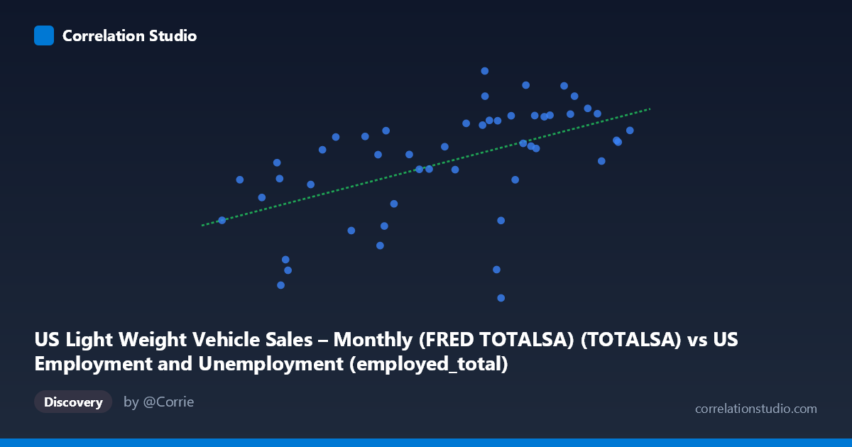
US Light Weight Vehicle Sales – Monthly (FRED TOTALSA) (TOTALSA) vs US Employment and Unemployment (employed_total)
- Pearson correlation (r)
- 0.5336
- Spearman correlation
- 0.5951
- p-value
- 0.000066
- Sample size (n)
- 50
- 95% confidence interval
- 0.2998 to 0.707
- Granger causality
- None
- Granger optimal lag
- 1
AI analysis
Analysis: US Light Vehicle Sales vs. Total Employment
1. Overall Relationship Revealed
The scatterplot reveals a moderate positive relationship between US Light Weight Vehicle Sales (X-axis, measured in thousands of units SAAR) and US Total Employment (Y-axis, in millions employed). As vehicle sales increase, total employment tends to rise as well, which is broadly intuitive — both indicators tend to expand during economic growth phases and contract during downturns. The linear regression equation (y = 5.33×10⁻⁵x + 8.14) captures this upward trend, though the considerable scatter around the regression line immediately signals that the relationship is far from deterministic and that many data points deviate substantially from the fitted line.
2. Correlation Strength, Direction, and Causality
The correlation coefficient of r = 0.517 indicates a moderate positive association, but the explanatory power is notably limited: R² = 0.267, meaning only about 26.7% of the variance in total employment is explained by light vehicle sales. The remaining ~73% is attributable to other factors entirely outside this model. The 95% confidence interval for r spans [0.279, 0.695], which is meaningfully wide — reflecting real uncertainty about the true population-level relationship, even with n = 50 paired observations from a population of N = 86 annual data points. The p-value of 0.00012 confirms the correlation is statistically significant and very unlikely to be a chance artifact. However, the Granger causality results are unambiguous in their null finding: neither direction (X→Y nor Y→X) reaches significance (F = 0.91, p = 0.344 and F = 0.71, p = 0.403, respectively). This means that past values of vehicle sales do not reliably predict future employment, and vice versa — the two series move together as contemporaneous co-indicators of economic conditions rather than one leading the other.
3. Notable Patterns, Clusters, and Outliers
Several features stand out in the data: - Lower-left cluster: Points around X = 88,000–105,000 with Y values spanning roughly 10.3–15.1 suggest that depressed auto sales periods (likely recessions, particularly 2008–2009) align with lower but still varied employment levels. - Notable outliers: The point (139,877; 9.79) is a clear anomaly — high vehicle sales paired with the lowest employment value in the dataset, suggesting a temporal mismatch or data alignment issue across the annual/monthly aggregation. Similarly, (99,526; 10.29) represents low sales and low employment, consistent with a deep recession year. - Upper-right diffusion: Higher sales values (140,000–163,000) show considerable vertical spread in employment (roughly 14–18.6 million range), indicating that at peak auto sales levels, employment varies substantially — the relationship weakens at higher values. - Non-linearity hint: The scatter pattern suggests potential saturation or heteroscedasticity at higher X values, where the variance in Y appears to increase, mildly violating linear regression assumptions.
4. Confounding Factors and Interpretation Caveats
Several important caveats apply to this correlation: - Shared business cycle dependency: Both variables are strongly driven by macroeconomic cycles (GDP growth, interest rates, consumer confidence). The correlation likely reflects common causation by the business cycle rather than any direct structural link between auto sales and employment. - Dataset mismatch: The X variable is monthly SAAR data from a vehicle sales dataset, while the Y variable is annual employment data from a labor dataset — the cross-dataset pairing introduces aggregation inconsistencies that could distort the measured relationship. - Temporal coverage (1976–2025): Spanning nearly 50 years introduces substantial structural breaks — shifts in the auto industry (foreign competition, EVs), labor market composition, and measurement methodologies all evolve over this period. - Reverse dataset labeling: Notably, the axis labels appear inverted relative to dataset sources (employment column appears in the vehicle sales dataset and vice versa), which warrants careful verification of the raw data alignment before drawing policy conclusions.
5. Actionable Insights and Further Investigation
Given these findings, several directions merit further exploration: - Decompose by economic regime: Segmenting the data into recession vs. expansion periods (using NBER recession dates) would clarify whether the correlation holds uniformly or is driven primarily by cyclical extremes. - Control for GDP or consumer confidence: Partial correlation analysis controlling for real GDP or the Consumer Confidence Index would reveal whether the vehicle–employment link is independent or entirely mediated by broader economic conditions. - Sector-specific employment: Rather than total employment, testing auto-manufacturing or durable goods employment specifically would provide a more theoretically grounded hypothesis — direct industry linkage rather than economy-wide co-movement. - Resolve the data alignment issue: The outlier at (139,877; 9.79) and the apparent dataset-label inversion should be investigated and corrected before any operational use of this regression model. - Lag structure exploration: Although Granger causality at lag-1 is insignificant, testing longer lag structures (2–4 periods) or using a Vector Autoregression (VAR) framework may reveal slower-moving predictive relationships between these series.
X dataset: US Employment and Unemployment
Y dataset: US Light Weight Vehicle Sales – Monthly (FRED TOTALSA)
Part of experiment: Yearly - US Employment and Unemployment vs US Light Weight Vehicle Sales – Monthly (FRED TOTALSA)