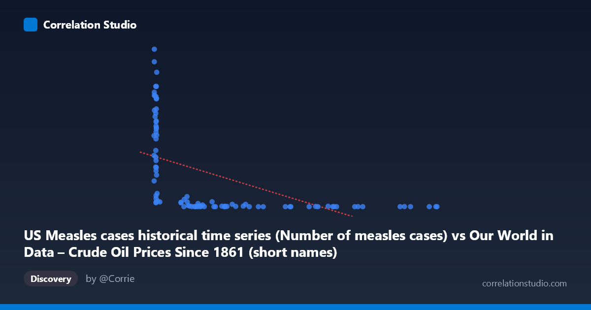
US Measles cases historical time series (Number of measles cases) vs Our World in Data – Crude Oil Prices Since 1861 (short names) (oil_price_crude_current_dollars_per_m3)
- Pearson correlation (r)
- -0.5384
- Spearman correlation
- -0.8514
- p-value
- 0
- Sample size (n)
- 92
- 95% confidence interval
- -0.6694 to -0.3749
- Granger causality
- None
- Granger optimal lag
- 10
AI analysis
Scatterplot Analysis: US Measles Cases vs. Crude Oil Prices
1. Overall Relationship Pattern
The scatterplot reveals a visually striking but statistically nuanced negative relationship between US measles cases and crude oil prices. Points are heavily concentrated at the low end of the X-axis (measles cases below ~200), where oil prices span an enormous range from near zero to over 800,000 cases-years, creating a pronounced L-shaped or hyperbolic distribution rather than a clean linear scatter. This immediately signals that a simple linear model is a poor geometric fit for the underlying data structure, even before examining the formal statistics.
2. Correlation Strength, Direction, and Causality
The Pearson r of −0.535 indicates a moderate negative correlation, but the r² of 0.286 is the more sobering figure — linear X explains only 28.6% of the variance in Y, leaving over 71% attributable to other factors. The 95% confidence interval of [−0.667, −0.370] is entirely negative and reasonably tight, and the p-value of 4.7×10⁻⁸ confirms this correlation is highly unlikely to be a sampling artifact. However, statistical significance here does not imply meaningful causation. Critically, the Granger causality test returns no significant directional predictability in either direction (X→Y: F=0.90, p=0.54; Y→X: F=1.35, p=0.23), meaning neither variable reliably predicts future values of the other in a temporal autoregressive framework. Furthermore, the note that Spearman ρ exceeds Pearson r confirms that the monotonic relationship is stronger than the linear one — a logarithmic or power-law transformation would almost certainly yield a better-fitting model.
3. Notable Patterns, Clusters, and Outliers
Several distinct structural features stand out:
- Dense left cluster: The majority of observations pile up at measles cases < 50, with oil prices ranging wildly from ~13 to ~894,000 — this cluster likely represents the post-vaccine era (post-1963) when measles was nearly eliminated but oil prices varied considerably across decades - High-Y outliers: Points like (7.17, 894,134), (7.11, 822,811), and (13.08, 763,094) represent extremely high measles case counts paired with very low oil prices, almost certainly corresponding to pre-vaccine decades (1920s–1950s) when both measles was endemic and oil was cheap - High-X, low-Y region: Points like (699.78, 220) and (702.38, 55) represent high oil prices with minimal measles cases — consistent with modern high-price oil eras where measles is effectively controlled - The data forms a classic confounded time-series arc rather than a mechanistically driven scatter
4. Confounding Factors and Interpretive Caveats
This correlation is an almost textbook example of spurious temporal correlation driven by a shared historical trend. Both variables are strongly time-dependent: measles cases plummeted after the 1963 vaccine introduction, while crude oil prices rose dramatically from the 1970s oil shocks onward and have continued inflating in nominal terms. These are parallel but causally unrelated secular trends — the negative correlation emerges because both series happened to move in opposite directions over the 20th century for entirely independent reasons. Additional caveats include:
- Nominal vs. real oil prices: Using nominal dollar figures introduces monetary inflation as a third confound - Population scaling: Measles cases are not normalized per capita, so U.S. population growth partially drives the denominator - Dataset labeling anomaly: The column labels appear swapped between datasets (measles data labeled as oil dataset and vice versa), warranting data provenance verification before any formal analysis - The Granger test used an optimal lag of 10 periods, which across a century-long annual series represents a decade — a span too large to reflect any plausible mechanism
5. Actionable Insights and Further Investigation
Given all of the above, the most important immediate action is to verify the dataset column assignments, as the axis labels suggest a possible metadata mismatch. Analytically, researchers should detrend both time series (e.g., first-differencing or residualizing against year) before computing correlations to strip out the shared temporal trend. A logarithmic transformation of Y (oil price) and a per-capita normalization of measles cases would produce a more statistically valid comparison. If the goal is genuine epidemiological or economic insight, partial correlation controlling for year would likely reduce r substantially toward zero, confirming the spurious nature of this association. This dataset pair serves as a valuable pedagogical example of why correlation + p-value alone are insufficient — temporal structure, causal plausibility, and effect size context (r² = 0.286) must all inform interpretation.
X dataset: Our World in Data – Crude Oil Prices Since 1861 (short names)
Y dataset: US Measles cases historical time series
Part of experiment: Yearly - Our World in Data – Crude Oil Prices Since 1861 (short names) vs US Measles cases historical time series