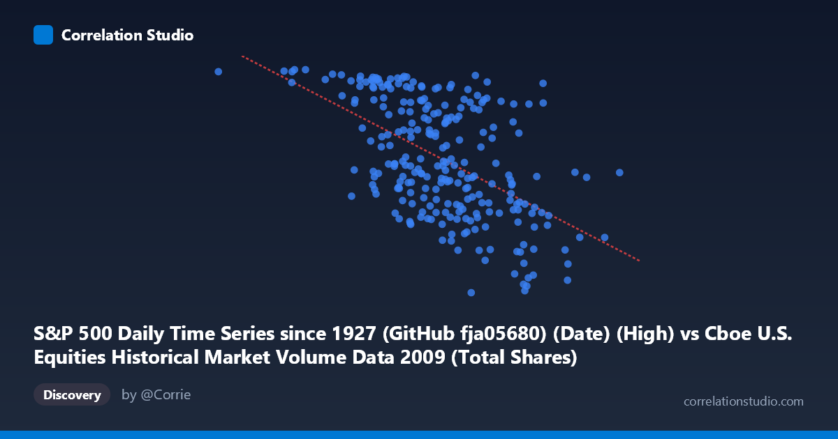
S&P 500 Daily Time Series since 1927 (GitHub fja05680) (Date) (High) vs Cboe U.S. Equities Historical Market Volume Data 2009 (Total Shares)
- Pearson correlation (r)
- -0.5448
- Spearman correlation
- -0.5397
- p-value
- 0
- Sample size (n)
- 252
- 95% confidence interval
- -0.6263 to -0.4517
- Granger causality
- X → Y
- Granger optimal lag
- 10
AI analysis
Scatterplot Analysis: S&P 500 Daily High vs. Cboe Total Shares Volume (2009)
Relationship Overview The scatterplot reveals a moderate negative relationship between the S&P 500 daily high price (X-axis) and total shares traded on U.S. equities exchanges (Y-axis) across 2009. As the S&P 500 daily high increases — moving from the crisis lows of early 2009 toward year-end recovery — total share volume tends to decline. This is consistent with a well-documented market dynamic: elevated trading volumes during periods of panic, uncertainty, and price discovery near market bottoms, followed by calmer, lower-volume trading as prices stabilize and recover. The linear regression equation (y = -3.95×10⁻⁷x + 1257.01) quantifies this inverse trend, though the scatter around the regression line is substantial.
Correlation Strength and Statistical Significance The Pearson correlation of r = -0.5448 indicates a moderate negative association, but the explanatory power is notably limited: R² = 0.2969, meaning only about 29.7% of the variance in total shares traded is explained by the S&P 500 daily high. The remaining ~70% of variance is attributable to other factors entirely. The 95% confidence interval of [-0.6263, -0.4517] is reasonably tight and does not include zero, and the p-value of effectively 0 confirms the result is highly statistically significant across the N = 3,232 population. Critically, the Granger causality analysis indicates a unidirectional relationship: X Granger-causes Y (F = 2.2960, p = 0.0140) at an optimal lag of 10 trading periods (approximately two calendar weeks), while the reverse direction fails significance (F = 1.7009, p = 0.0818). This suggests that S&P 500 price levels have modest but statistically meaningful predictive power over future trading volume, not the other way around — a practically useful directional finding.
Notable Patterns, Clusters, and Outliers The data exhibits a distinctive funnel or heteroscedastic shape: at lower X values (S&P 500 highs in the ~200M–600M range, corresponding to early 2009 crisis conditions), Y values (share volume) are highly dispersed, ranging from roughly 800 to over 1,130 billion shares. As X increases toward year-end recovery levels (900M–1.2B range), the Y distribution tightens considerably and trends lower. Several noteworthy outliers are visible: the point near (192M, 1126) represents an extreme low-price, high-volume session consistent with the market bottom period, while (1212M, 930) at the far right represents a high-price, moderate-volume late-year session. A cluster of points around (950M–1,000M, 700–800) suggests particularly low-volume sessions during the mid-recovery phase, potentially holiday-adjacent or low-liquidity trading days.
Confounding Factors and Caveats Several important caveats temper this interpretation. First, the X-axis label appears to contain a units mismatch — the X range (192M to 1.2B) labeled as "Date (High)" from the S&P 500 dataset is unusual for price values, suggesting possible data alignment or labeling issues worth verifying. Second, 2009 is a structurally unique year — spanning the global financial crisis trough (March 2009 S&P bottom ~666) through a 60%+ recovery — making this correlation potentially regime-specific and non-generalizable to normal market years. Third, the negative correlation likely reflects a common underlying driver: macroeconomic fear and volatility (e.g., VIX levels) simultaneously depressed prices and inflated volumes, making the relationship partially or wholly spurious in causal terms beyond what Granger analysis captures. The Granger lag of 10 periods also warrants caution — it reflects statistical precedence, not necessarily economic causation.
Actionable Insights and Further Investigation The 10-period Granger lag finding is the most practically actionable result: traders and analysts monitoring S&P 500 price trends may gain ~2-week forward-looking signal about aggregate market volume conditions, which has implications for liquidity forecasting and execution strategy. However, given that only 29.7% of variance is explained, this signal should be combined with other predictors. Recommended next steps include: (1) incorporating VIX or implied volatility as a mediating variable to test whether it absorbs the price-volume relationship; (2) extending the analysis across multiple years to assess whether the negative correlation holds in bull market years or is specific to crisis-recovery dynamics; (3) conducting a rolling-window correlation analysis to identify whether the relationship strengthens near volatility regimes; and (4) resolving the apparent data labeling ambiguity on the X-axis to confirm the variable being measured is indeed S&P 500 daily high price in standard units.
X dataset: Cboe U.S. Equities Historical Market Volume Data 2009
Y dataset: S&P 500 Daily Time Series since 1927 (GitHub fja05680) (Date)
Part of experiment: Daily - Cboe U.S. Equities Historical Market Volume Data 2009 vs S&P 500 Daily Time Series since 1927 (GitHub fja05680) (Date)