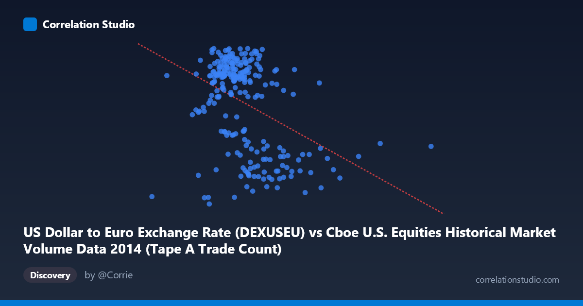
US Dollar to Euro Exchange Rate (DEXUSEU) vs Cboe U.S. Equities Historical Market Volume Data 2014 (Tape A Trade Count)
- Pearson correlation (r)
- -0.4003
- Spearman correlation
- -0.3351
- p-value
- 0
- Sample size (n)
- 249
- 95% confidence interval
- -0.4998 to -0.2904
- Granger causality
- None
- Granger optimal lag
- 1
AI analysis
Scatterplot Analysis: USD/EUR Exchange Rate vs. Cboe Tape A Trade Count (2014)
Relationship Overview
The scatterplot reveals a moderate negative relationship between the US Dollar to Euro exchange rate and Cboe Tape A trade counts during 2014. As the exchange rate increases (USD strengthening relative to EUR), trade counts tend to decrease, and vice versa. The linear regression equation (y = -9.09E-08x + 1.437) captures this downward slope, though the scatter around the regression line is substantial, indicating that the relationship is real but far from deterministic. The data points span a meaningful range on both axes, with trade counts clustering between roughly 1.21–1.39 and volume figures spanning approximately 527K to 2.5M.
Correlation Strength and Statistical Significance
The Pearson correlation of r = -0.40 indicates a moderate negative association, but the more informative metric is r² = 0.1602, meaning only 16% of the variance in Tape A trade counts is explained by the USD/EUR exchange rate. The remaining 84% of variation is attributable to other factors entirely. The 95% confidence interval of [-0.50, -0.29] is meaningfully negative throughout, and the p-value of 5.33E-11 confirms this correlation is highly statistically significant given the sample (n=249) and population (N=3,686). However, statistical significance should not be conflated with practical importance — a 16% explanatory share is modest. Crucially, Granger causality testing finds no significant predictive directionality in either direction (X→Y: p=0.897; Y→X: p=0.364), meaning neither variable reliably predicts the other in a temporal lead-lag framework. The correlation may be contemporaneous or driven by shared underlying forces rather than any causal pathway.
Patterns, Clusters, and Outliers
Several notable structural features are visible in the data. There is a dense central cluster of points concentrated between roughly 1,000,000–1,250,000 on the X-axis and 1.34–1.39 on the Y-axis, suggesting that most trading days in 2014 fell within a fairly narrow band of both metrics. A secondary, visually distinct lower cluster appears around Y-values of 1.23–1.25, representing days with notably lower USD/EUR rates, and these points tend to appear at higher X values, reinforcing the negative slope. There are several high-volume outliers extending toward 2.0M–2.5M on the X-axis, likely corresponding to high-volatility market events such as geopolitical shocks or FOMC announcements. These extreme X values are sparse and may exert disproportionate leverage on the regression coefficient.
Confounding Factors and Caveats
Several important caveats apply to this analysis. First, reverse axis labeling deserves attention — the dataset descriptions appear swapped in metadata (X is labeled as exchange rate data sourced from Cboe volume data, and vice versa), which could reflect a data joining artifact and warrants verification. Second, both variables are likely driven by common macroeconomic factors in 2014, including Federal Reserve tapering decisions, European Central Bank monetary easing, and geopolitical events such as the Russia-Ukraine conflict — all of which could simultaneously affect both currency markets and equity trading volumes, creating a spurious correlation. Third, temporal autocorrelation within daily financial time series is almost certain, which may inflate the effective sample size and the apparent statistical significance. Finally, the relationship may be non-stationary, with the correlation structure shifting across different market regimes within the year.
Actionable Insights and Further Investigation
Despite modest explanatory power, these findings suggest several productive avenues. Analysts should segment the data by quarter or market regime to assess whether the correlation strengthens during specific periods, such as high-volatility windows driven by ECB policy announcements. It would be valuable to introduce additional covariates — VIX levels, S&P 500 returns, Fed funds futures — in a multivariate model to determine whether the exchange rate retains explanatory power after controlling for broader market conditions. Given the Granger causality null results, researchers should test for contemporaneous relationships using same-day event studies around key macro announcements. Finally, applying cointegration testing would help determine whether any long-run equilibrium relationship exists between these series beyond the short-term daily correlation observed here.
X dataset: Cboe U.S. Equities Historical Market Volume Data 2014
Y dataset: US Dollar to Euro Exchange Rate
Part of experiment: Daily - Cboe U.S. Equities Historical Market Volume Data 2014 vs US Dollar to Euro Exchange Rate