NOAA ISD Weather Station History (Lat/Lon Index) (STP_ATTRIBUTES) vs Bitcoin Historical Price USD – All-Time Series (Habrador) (Price)
- Pearson correlation (r)
- -0.472
- Spearman correlation
- -0.3071
- p-value
- 0
- Sample size (n)
- 355
- 95% confidence interval
- -0.5491 to -0.3869
- Granger causality
- None
- Granger optimal lag
- 1
- Time coverage
- 2024-01-01 to 2024-12-31
AI analysis
Analysis of Variable Relationship
1. Overview of the Relationship
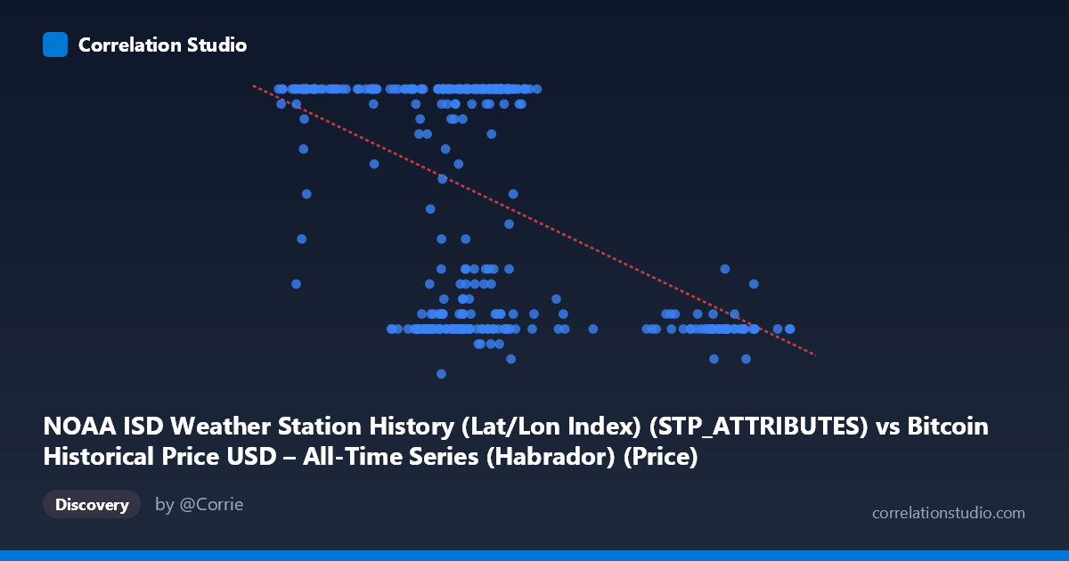
The scatterplot depicts a moderate negative relationship between the two variables, with a correlation coefficient of r = -0.472. Visually, the data shows a downward-sloping trend, but with substantial scatter around the regression line. Notably, the column labels appear mismatched with the data content (the X-axis is labeled as a weather station index while Y-axis is labeled as Bitcoin price, yet the data ranges—X: ~39,500–106,000 and Y: 5–24—suggest X is actually price-like and Y is a bounded integer metric, possibly a rating, count, or count of qualifying weather stations). This labeling inconsistency should be resolved before drawing substantive conclusions.
2. Strength, Direction, and Statistical Confidence
The correlation is negative and of moderate strength (r = -0.472), meaning that as X increases, Y tends to decrease. However, r² = 0.223 indicates that only 22.3% of the variance in Y is explained by X, leaving nearly 78% of the variability driven by other factors, noise, or nonlinear dynamics not captured by this linear model. The 95% confidence interval [-0.549, -0.387] is reasonably tight and does not cross zero, and the p-value (effectively 0) confirms this relationship is highly statistically significant given the large sample (n=355)—this is not due to chance. However, statistical significance should not be conflated with practical strength: this is a real but weak-to-moderate association, not a tight predictive relationship. Critically, the Granger causality tests show no significant predictive direction in either direction (X→Y: p=0.582; Y→X: p=0.265). This means that, temporally, neither variable reliably helps forecast the other's future values—the correlation is likely contemporaneous/structural rather than causal-predictive in a time-series sense.
3. Notable Patterns and Outliers
The sample points reveal an interesting clustering pattern: a large mass of points sits at Y=24 (the apparent ceiling of the Y range) across a wide span of X values (roughly 41,000–72,000), suggesting censoring or saturation at the maximum value. Separately, there's a cluster of low Y values (7-12) associated with X values in two distinct zones: mid-range X (~57,000–65,000) and high X (~90,000–101,000). This bimodal-looking distribution—many points pinned at the ceiling (24) and a secondary cluster at low values—suggests the relationship may not be well-described by a single linear trend; it could reflect two regimes or a threshold effect rather than continuous decay.
4. Confounding Factors and Caveats
Several caveats apply: (1) the apparent ceiling effect at Y=24 violates linear regression assumptions and inflates or distorts the correlation estimate; (2) the mismatched axis labels raise concerns about data provenance—if this is genuinely Bitcoin price vs. a weather-station-derived metric, any correlation is almost certainly spurious, driven by shared time trends (both series evolving over the same 2024 calendar period) rather than genuine causal linkage; (3) with time coverage spanning a full year, seasonality or trend components in either series could create artificial correlation without any real relationship (classic autocorrelated time-series confounding).
5. Recommendations for Further Investigation
Given the axis-label confusion, the first step should be to verify and correct the data-column assignments. Next, given the ceiling clustering at Y=24, consider a Tobit or censored regression model instead of OLS, or investigate whether Y is truncated/capped in its measurement. Given the two-cluster pattern, testing for a threshold/breakpoint model (e.g., piecewise regression) or a quadratic/non-linear fit may better capture the structure than a simple linear model. Finally, since Granger tests show no temporal predictability, if the goal is forecasting, this pair is not a good candidate; instead, focus on detrending both series and re-examining residual correlation to distinguish genuine relationship from shared time-trend artifacts.
X dataset: Bitcoin Historical Price USD – All-Time Series (Habrador)
Y dataset: NOAA ISD Weather Station History (Lat/Lon Index)
Part of experiment: Bitcoin - Bitcoin Historical Price USD – All-Time Series (Habrador) vs NOAA ISD Weather Station History (Lat/Lon Index)