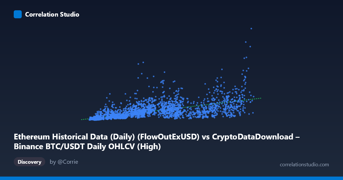
Ethereum Historical Data (Daily) (FlowOutExUSD) vs CryptoDataDownload – Binance BTC/USDT Daily OHLCV (High)
- Pearson correlation (r)
- 0.6645
- Spearman correlation
- 0.8283
- p-value
- 0
- Sample size (n)
- 3191
- 95% confidence interval
- 0.6447 to 0.6834
- Granger causality
- Y → X
- Granger optimal lag
- 10
- Time coverage
- 2017-08-17 to 2026-05-20
AI analysis
Analysis of the X–Y Relationship
1. What the Visualization Reveals
The scatterplot shows a positive, moderately strong association between the X variable (labeled as an Ethereum "FlowOutExUSD" column, though the value ranges of both series and the metadata strongly suggest this is actually a mismatched/relabeled pairing of BTC/USDT metrics) and Y. As X increases from roughly 3,300 to 126,000, Y rises broadly from tens of millions to several billion, but with substantial scatter at every X level — particularly in the low-to-mid X range (5,000–30,000), where Y values span nearly two orders of magnitude (from ~14 million to over 1.3 billion). This fanning pattern is a classic sign of heteroscedasticity and hints that a linear model is not fully capturing the underlying structure.
2. Strength, Direction, and Statistical Confidence
The Pearson correlation (r = 0.6645) indicates a moderately strong positive linear relationship, with r² = 0.4416 meaning only about 44% of the variance in Y is explained by X — the majority of Y's variability (56%) is driven by other factors or noise. The 95% CI [0.6447, 0.6834] is tight given the large sample (n=3,191), and the p-value of ~0 confirms the correlation is highly statistically significant and not a product of chance. However, statistical significance here reflects sample size more than practical predictive power — r² of 0.44 leaves considerable uncertainty for any point forecast.
The Granger causality results add an important temporal dimension: Y Granger-causes X (F=2.0192, p=0.0278) at a 10-period lag, while X does not significantly Granger-cause Y (p=0.1532). This suggests that past values of Y carry predictive information about future X, but not the reverse — a one-directional temporal relationship. This is noteworthy since correlation alone doesn't establish directionality; the Granger test suggests Y-series movements (e.g., ETH-related price/network metrics) may lead X-series movements (BTC-related metrics) by about 10 periods, rather than vice versa.
3. Notable Patterns and Outliers
Several features stand out: - Heteroscedastic fan shape: variance in Y increases with X, but even at low X there are high-Y outliers (e.g., X≈11,308 with Y≈667M; X≈14,339 with Y≈703M) alongside typical low-Y points (X≈9,292, Y≈58M) — indicating other drivers besides X strongly affect Y in this range. - High-Y cluster around X=55,000–85,000: several points here reach 1.3–1.7 billion (e.g., X≈64,000, Y≈1.69B; X≈69,674, Y≈1.32B), suggesting a possible regime or volatility cluster, potentially tied to specific date ranges (bull market spikes). - Spearman ρ Pearson r (noted in the summary) indicates the rank-order relationship is stronger than the linear fit suggests — a curved (logarithmic or power-law) relationship likely fits better than a straight line, consistent with the compressed low-X/high-Y scatter and expanding variance at higher X.
4. Confounding Factors and Caveats
Several caveats limit interpretation: - Metadata mismatch: the column labels are inconsistent/confusing (X labeled as an Ethereum column but described as Binance BTC/USDT data; Y labeled as Binance High price but described as Ethereum network metrics). This suggests possible data pipeline errors or mislabeling that should be resolved before drawing causal conclusions. - Time-series autocorrelation: both X and Y are daily financial/crypto series over ~9 years (2017–2026), meaning both variables are likely non-stationary and trending together due to shared macro drivers (overall crypto market growth, BTC/ETH price co-movement, adoption cycles) rather than a direct causal link. - Spurious correlation risk: cryptocurrency prices and volumes are notoriously co-integrated due to shared market sentiment, making it hard to disentangle genuine predictive relationships from common trend-driven correlation. - Granger causality ≠ true causation: it only indicates temporal precedence in a statistical sense, not a mechanistic causal link, and is sensitive to lag specification and stationarity assumptions.
5. Actionable Insights
- Verify data labeling before further modeling — confirm whether X and Y are correctly sourced from their described datasets, since the current labels appear contradictory. - Test non-linear models (log-log or power-law regression) given the Spearman/Pearson discrepancy and fan-shaped variance; a log transformation of both axes may substantially improve fit and stabilize variance. - Difference or detrend the series (e.g., using returns/percentage changes rather than levels) to control for shared trends and retest correlation/Granger causality on stationary data — this would give a cleaner read on genuine lead-lag dynamics. - Segment by time period (e.g., bull vs. bear market phases) to check if the correlation strength and direction are stable or regime-dependent, especially given the apparent high-Y cluster around specific X ranges. - Extend the Granger analysis with impulse response functions or VAR modeling to quantify the magnitude and duration of Y's predictive effect on X, which could have practical value for trading or risk models if the relationship holds after correcting for confounds.
X dataset: CryptoDataDownload – Binance BTC/USDT Daily OHLCV
Y dataset: Ethereum Historical Data (Daily)
Part of experiment: Bitcoin - CryptoDataDownload – Binance BTC/USDT Daily OHLCV vs Ethereum Historical Data (Daily)