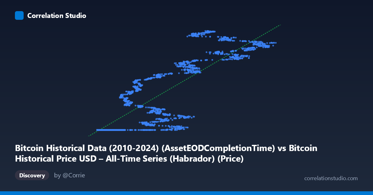
Bitcoin Historical Data (2010-2024) (AssetEODCompletionTime) vs Bitcoin Historical Price USD – All-Time Series (Habrador) (Price)
- Pearson correlation (r)
- 0.893
- Spearman correlation
- 0.9723
- p-value
- 0
- Sample size (n)
- 5789
- 95% confidence interval
- 0.8877 to 0.8981
- Granger causality
- None
- Granger optimal lag
- 10
- Time coverage
- 2010-07-18 to 2026-05-23
- Recomputed on refreshed data
- 2026-10-24 (r was 0.8924)
AI analysis
Analysis: Bitcoin "Completion Time" Column vs. Bitcoin Price
1. What the Visualization Reveals
This scatterplot is somewhat unusual in that both axes derive from the same underlying dataset (Bitcoin's historical price series), but the X-axis is actually a mislabeled or repurposed field — "AssetEODCompletionTime" — being treated as a numeric index rather than a genuine independent variable. The values range from near-zero (0.05) to ~124,720, which looks more like a row index, elapsed time unit, or processing artifact than a meaningful economic variable. The scatter shows a clustering pattern: many points sit at low X values (0–1,000) with Y values compressed near the dataset minimum (~1.614 billion), while higher X values spread Y across a much wider range up to the maximum (~1.777 billion). This is consistent with X behaving as a rough proxy for chronological sequence/time rather than a causal driver of price.
2. Correlation Strength and Statistical Confidence
The correlation coefficient (r = 0.892, r² = 0.796) indicates a strong positive linear relationship, with the linear regression explaining 79.6% of the variance in Y. The 95% CI [0.887, 0.898] is tight, and the p-value of ~0 confirms this relationship is not due to chance — with n = 5,764, even modest correlations would be significant, but this effect size is substantial. However, the Granger causality results are critical: neither direction (X→Y or Y→X) shows significant predictive causality (p = 0.78 and 0.76, both far above 0.05). This means that despite the strong contemporaneous correlation, X does not temporally precede or forecast changes in Y, nor vice versa. Practically, this tells us the relationship is likely a shared trend or index artifact rather than a genuine predictive/causal linkage — the correlation is descriptive, not forecastable.
3. Notable Patterns and Non-Linear Features
The sample points reveal a non-linear, heteroscedastic structure: at low X (under ~1,000), Y is tightly clustered near 1.614B regardless of X value — suggesting many early rows/timestamps correspond to Bitcoin's early low-price era. As X increases beyond ~20,000, Y values fan out dramatically (ranging from 1.615B to 1.777B) even for similar X values (e.g., X≈26,900 gives Y=1.684B in one instance and Y=1.697B in another; X≈42,992 vs 44,118 gives 1.707B vs 1.644B). This "widening funnel" pattern indicates increasing variance at higher X — a classic sign that a simple linear fit understates the complexity of the relationship, and that log-transformation or a piecewise/non-linear model would fit better. There also appear to be near-vertical clusters (many rows sharing similar X but different Y), suggesting X may not be finely granular or continuous.
4. Confounding Factors and Caveats
The most important caveat: this is very likely a spurious or artifactual correlation driven by shared temporal ordering, not an economic relationship. If X represents a completion-time index or row sequence, then correlating it with price simply reflects Bitcoin's long-term upward price trend over the 2010–2026 window — any monotonically increasing index will correlate with a generally rising price series. The Granger non-causality result reinforces this: there's no lead-lag structure, just co-trending. Additionally, Bitcoin's known volatility clustering, bubble cycles (2013, 2017, 2021), and structural breaks mean a single linear model is a poor description of the true dynamics — the r² is inflated by the dominant long-term trend while masking cyclical crashes and rallies.
5. Suggested Next Steps
1. Clarify the true meaning of the X variable — confirm whether "AssetEODCompletionTime" is a timestamp, row index, or processing duration; if it's a disguised time variable, replace it with actual calendar time for proper time-series analysis. 2. Detrend or difference both series (e.g., use returns/log-returns instead of levels) before assessing correlation — this will reveal whether any genuine relationship survives after removing the shared trend. 3. Segment by market regime (bull/bear cycles) to check if the relationship is stable or driven entirely by specific periods (e.g., 2021 and 2024 bull runs visible in the high-X, high-Y samples). 4. Re-run Granger causality on stationary (differenced) series, since the current non-significant result may partly reflect non-stationarity in both series rather than true absence of predictive power.
X dataset: Bitcoin Historical Price USD – All-Time Series (Habrador)
Y dataset: Bitcoin Historical Data (2010-2024)
Part of experiment: Bitcoin - Bitcoin Historical Price USD – All-Time Series (Habrador) vs Bitcoin Historical Data (2010-2024)