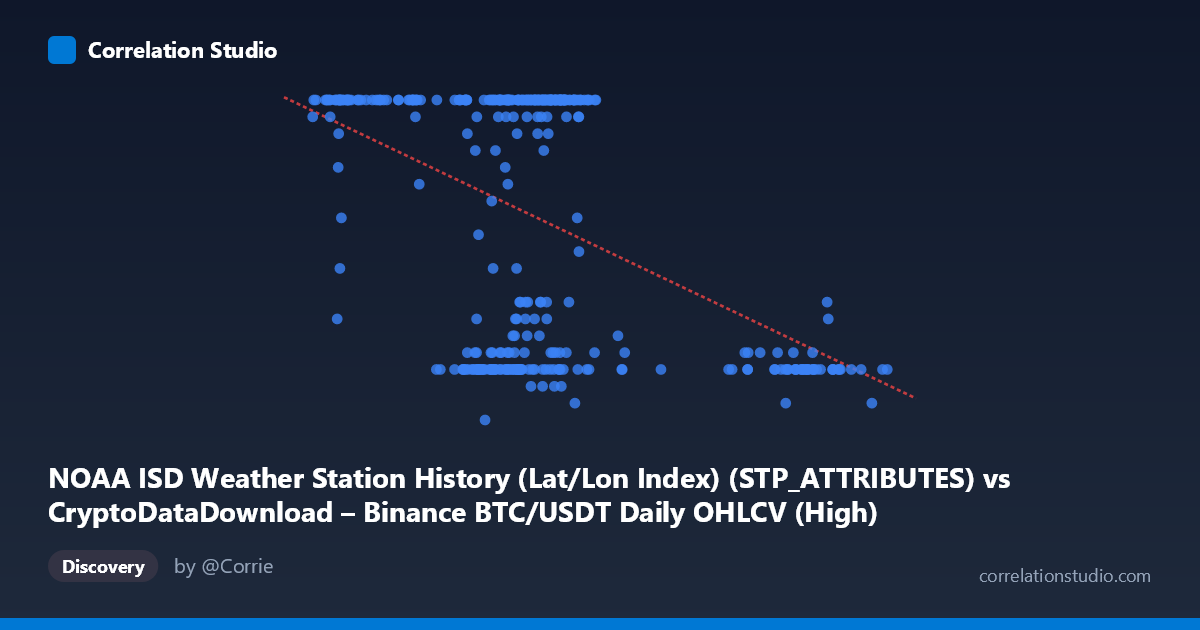
NOAA ISD Weather Station History (Lat/Lon Index) (STP_ATTRIBUTES) vs CryptoDataDownload – Binance BTC/USDT Daily OHLCV (High)
- Pearson correlation (r)
- -0.4673
- Spearman correlation
- -0.2953
- p-value
- 0
- Sample size (n)
- 355
- 95% confidence interval
- -0.5449 to -0.3818
- Granger causality
- None
- Granger optimal lag
- 1
AI analysis
Scatterplot Analysis: X (Weather Station Index) vs Y (BTC/USDT High)
Note on variable labeling: The axis metadata appears swapped/mismatched — the X-axis is labeled as a NOAA station attribute but contains values (~40,000–108,000) consistent with a BTC/USDT price-like series, while Y (5–24) looks more like a bounded index or scaled value than a raw "High" price. This mismatch should be resolved before drawing substantive conclusions, but the analysis below addresses the statistical relationship as given.
1. What the Visualization Reveals The scatterplot shows a moderate negative linear trend: as X increases, Y tends to decrease, following the fitted line y = -0.000238x + 32.93. However, the relationship is far from clean — Y is heavily concentrated at two levels (values clustering near 8-9 and near 24), suggesting Y may be a discretized, categorical, or capped variable rather than a smooth continuous measurement. This bimodal clustering is the dominant visual feature, with the negative slope emerging as an aggregate trend across these two bands rather than a tight continuous decay.
2. Strength, Direction, and Uncertainty - Correlation (r = -0.467) indicates a moderate negative association. - R² = 0.218 means only about 22% of the variance in Y is explained by X — roughly 78% of Y's variability is driven by other factors, noise, or non-linear structure not captured by this linear model. - The 95% CI [-0.545, -0.382] is fairly narrow and entirely negative, and the p-value ≈ 0 confirms the correlation is statistically robust and not due to chance, despite the large N (355). - Practical takeaway: the relationship is real but weak-to-moderate in explanatory power — useful as a directional signal, not as a predictive model on its own. - Granger causality shows no significant predictive direction either way (X→Y: p=0.71; Y→X: p=0.23). This means neither variable's past values help forecast the other's future values at lag 1 — the correlation is likely contemporaneous/structural rather than causal or lead-lag in nature.
3. Notable Patterns and Outliers - The data shows a strong bimodal Y distribution: a dense cluster at Y≈24 (the ceiling) spanning most of the X range, and a secondary cluster at Y≈8-12, concentrated at higher X values (60,000-70,000+ and especially X90,000). - This creates a step-like or threshold pattern: below certain X ranges, Y is almost always at its maximum (24); above ~90,000, Y drops sharply to single digits. This looks more like a regime shift or saturation effect than a linear relationship — the linear r/R² substantially understates this structural break. - Points like (98564, 8), (98270, 8), (91449.99, 9) suggest a cluster of high-X/low-Y outliers distinct from the main cloud.
4. Confounding Factors and Caveats - Metadata mismatch (as noted) raises concern that this may be a spurious or mismatched pairing of unrelated series (crypto price data vs. weather station attributes) — a classic risk of automated correlation pipelines discovering coincidental patterns in unrelated time series. - Y's apparent ceiling/floor behavior (repeated exact values of 24, 8, 9) suggests it may be a bucketed, categorical, or capped index (e.g., an hour, a score, or a day-count) rather than a continuous physical quantity — linear correlation metrics are not well-suited to such data. - With time coverage of a full year (2024), any shared seasonal trend or autocorrelation in both series could produce a spurious correlation without genuine causal linkage.
5. Recommendations for Further Investigation - Verify the data pipeline/column mapping — confirm that X and Y are correctly sourced from their intended datasets before further modeling. - Given the bimodal Y pattern, consider logistic regression or classification (Y high vs. low) rather than linear regression, or a piecewise/threshold model around X≈90,000. - Test for seasonality in both series independently (e.g., decompose by month) to rule out spurious correlation from shared trends. - Since Granger tests show no lead-lag relationship, treat this as a cross-sectional/contemporaneous association only — not suitable for forecasting one variable from the other's history.
X dataset: CryptoDataDownload – Binance BTC/USDT Daily OHLCV
Y dataset: NOAA ISD Weather Station History (Lat/Lon Index)
Part of experiment: Bitcoin - CryptoDataDownload – Binance BTC/USDT Daily OHLCV vs NOAA ISD Weather Station History (Lat/Lon Index)