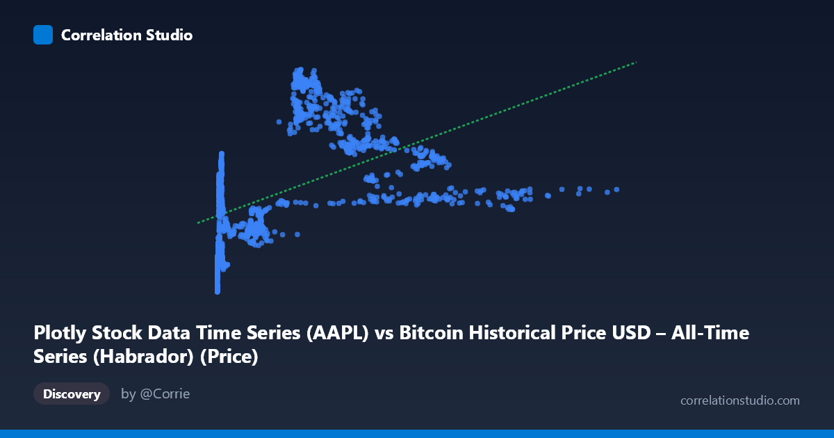
Plotly Stock Data Time Series (AAPL) vs Bitcoin Historical Price USD – All-Time Series (Habrador) (Price)
- Pearson correlation (r)
- 0.4869
- Spearman correlation
- 0.7008
- p-value
- 0
- Sample size (n)
- 1415
- 95% confidence interval
- 0.4461 to 0.5257
- Granger causality
- X → Y
- Granger optimal lag
- 1
AI analysis
Analysis: Bitcoin Price Series vs. Stock Data Time Series
Note on labels: The axis metadata appears swapped/mismatched (X is labeled as "AAPL" data but described as Bitcoin price history, while Y is labeled "Bitcoin" but described as stock data). Given the actual value ranges — X spans 0.05 to 1147.25 (consistent with early Bitcoin prices) and Y spans 31.74 to 130.67 (consistent with a stock price like AAPL in this era) — this analysis treats X as Bitcoin price and Y as the equity/stock price, which aligns with the numeric distributions regardless of the dataset naming.
1. What the Visualization Reveals The scatterplot shows a positive but non-linear relationship between the two price series. Sample points illustrate a steep initial climb: as X moves from near-zero to roughly 300, Y rises sharply from the 30s/40s up into the 110-130 range. Beyond X≈300, the relationship flattens and even reverses somewhat — Y values cluster in the 70-100 range across a wide X spread (300 to 1147), with no further systematic increase. This produces a curved, saturating pattern rather than a straight line, consistent with the note that Spearman's rank correlation exceeds Pearson's r.
2. Strength, Direction, and Predictive Direction The linear Pearson correlation (r = 0.487, R² = 0.237) indicates a moderate positive association, but explains only about 24% of the variance in Y — the majority of Y's movement is driven by other factors or non-linear dynamics not captured by this simple linear fit. The 95% CI [0.446, 0.526] is tight and the p-value is effectively zero, so we can be confident the true correlation is non-zero and positive — but confidence in the existence of a relationship should not be conflated with the relationship being strong or linear. The Granger causality test adds a temporal dimension: X leads Y at a 1-period lag (F = 6.95, p = 0.0085) while Y does not predict X (p = 0.588). This suggests a unidirectional, time-lagged predictive relationship — historical values of X carry information useful for forecasting Y, but not vice versa. This is a statistical predictive relationship, not proof of causal mechanism.
3. Notable Patterns and Outliers The data shows a clear two-regime structure: a rapid-growth phase at low X values (X < 100) where Y climbs steeply with X, and a plateau/saturation phase at higher X values where Y oscillates in a narrower band (roughly 70-100) independent of further X increases. The dense cluster near X≈0-15 with Y spanning 32-86 suggests high sensitivity/volatility in Y during this low-X regime. Points like (237.33, 127.79) and (290.88, 123.89) represent local peaks in Y that don't correspond to the highest X values, hinting at a hump-shaped or logarithmic curve rather than monotonic growth. The largest X values (600-1147) correspond to comparatively modest, even declining, Y values, reinforcing the non-linear/saturating shape.
4. Confounding Factors and Caveats Both series are financial time series covering overlapping periods (2010-2016), meaning both are subject to shared macroeconomic trends, market sentiment, and time-based autocorrelation — a classic confound in time-series correlation. Neither series is stationary, so the correlation may partly reflect co-trending rather than a genuine functional relationship (spurious correlation risk). The Granger result, while suggestive of lead-lag dynamics, is also vulnerable to this same non-stationarity issue and reverse-causality omitted variables (e.g., broader market indices, USD strength, or macro news events) could independently drive both series.
5. Suggested Next Steps 1. Fit non-linear models — logarithmic (Y ~ log(X)) or polynomial regression given the Spearman/Pearson divergence and visible saturation curve. 2. Difference or detrend both series (e.g., use returns/percent changes instead of raw prices) before re-running correlation and Granger tests to rule out spurious trend-driven correlation. 3. Segment the analysis by regime (low-X rapid growth vs. high-X plateau) to check if the relationship strength/direction differs structurally. 4. Control for time/date directly and test partial correlation controlling for a common macro factor. 5. Validate the Granger result with additional lag structures and out-of-sample forecasting tests before treating X as a practical leading indicator for Y.
X dataset: Bitcoin Historical Price USD – All-Time Series (Habrador)
Y dataset: Plotly Stock Data Time Series
Part of experiment: Bitcoin - Bitcoin Historical Price USD – All-Time Series (Habrador) vs Plotly Stock Data Time Series