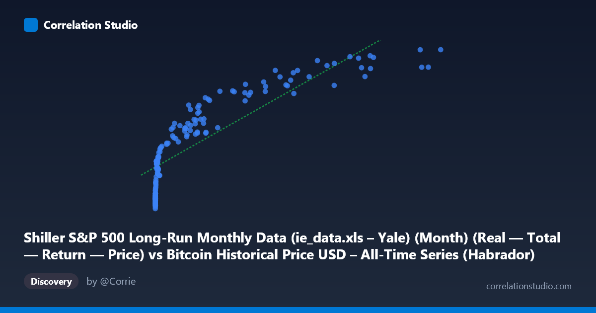
Shiller S&P 500 Long-Run Monthly Data (ie_data.xls – Yale) (Month) (Real — Total — Return — Price) vs Bitcoin Historical Price USD – All-Time Series (Habrador) (Price)
- Pearson correlation (r)
- 0.8591
- Spearman correlation
- 0.9731
- p-value
- 0
- Sample size (n)
- 158
- 95% confidence interval
- 0.8118 to 0.8951
- Granger causality
- None
- Granger optimal lag
- 10
- Time coverage
- 2010-08-01 to 2023-09-01
- Recomputed on refreshed data
- 2026-10-10 (r was 0.8591)
AI analysis
Analysis: Bitcoin Price vs. S&P 500 (Shiller Data)
1. What the Visualization Reveals
The scatterplot shows a strong positive association between Bitcoin's price trajectory and the Shiller S&P 500 series, but the shape of the relationship is distinctly non-linear. At low X-values (roughly 0–1,000), Y values span an enormous range (~830,000 to ~1,740,000), indicating a steep, compressed initial rise. As X increases into the tens of thousands, Y growth flattens considerably — the data has the classic concave, logarithmic-like curve rather than a straight line. This is reinforced by the note that Spearman's ρ exceeds Pearson's r, meaning the rank-order relationship is even stronger than the linear one, a hallmark signature of a monotonic but curved relationship.
2. Strength, Direction, and Uncertainty
The Pearson correlation (r = 0.859) is strong and positive, with r² = 0.738 indicating that a linear model explains about 74% of the variance in Y — substantial, but leaving over a quarter of variance unexplained, likely due to the curvature noted above. The 95% CI [0.812, 0.895] is tight and does not cross zero, and the p-value is effectively 0, so we can be confident this correlation is not a statistical fluke within this sample. However, Granger causality tests show no significant predictive direction in either direction (X→Y p=0.546; Y→X p=0.486). This is a critical caveat: despite the strong contemporaneous correlation, neither series helps forecast the other's future values based on past lags. This strongly suggests the relationship is not causal in a temporal-predictive sense — it's more likely that both series share a common underlying driver (e.g., time itself, monotonic growth trends, or macro liquidity conditions) rather than one directly leading the other.
3. Notable Patterns and Outliers
The data clearly separates into two regimes: a "low-X cluster" (X < 1,000) where Y ranges tightly between ~830K–1.74M, and a "high-X cluster" (X 5,000) where Y climbs toward 2.4M–3.2M with more scatter. The transition zone (X ≈ 1,000–5,000) shows a rapid vertical climb in Y with relatively small changes in X — this is the steepest part of the curve and likely corresponds to Bitcoin's explosive early growth phases. At the high end, points like (46,208, 3,192,049) and (46,281, 2,990,780) show Y actually plateauing or even dipping slightly despite rising X, suggesting saturation or independent volatility in Y unrelated to X at that range.
4. Confounding Factors and Caveats
Both series are monotonically trending over the same 2010–2023 time window, which is a classic setup for spurious correlation via a shared time trend — two unrelated trending series will show high correlation simply because both increase over time. The lack of Granger causality supports this concern: the relationship may be an artifact of common temporal drift rather than genuine economic linkage. Additionally, Bitcoin's price is denominated in raw USD with extreme scale differences (0.06 to 61,374), meaning the regression is highly sensitive to compression/expansion effects at different scales — a log transformation would likely be far more appropriate than the current linear fit.
5. Suggested Next Steps
1. Re-fit using log(X) or log(Y) (or both) given the strong log-like curvature and Spearman Pearson signal — this should substantially improve explained variance. 2. De-trend both series (e.g., first-differencing or removing time trend) before assessing correlation, to rule out spurious trend-driven correlation. 3. Re-run Granger causality on de-trended/differenced series — the current non-significant result may change once shared trend is removed, revealing (or ruling out) genuine lead-lag dynamics. 4. Treat this relationship as descriptive/correlational only — it should not be used for forecasting one series from the other given the null causality result.
X dataset: Bitcoin Historical Price USD – All-Time Series (Habrador)
Y dataset: Shiller S&P 500 Long-Run Monthly Data (ie_data.xls – Yale) (Month)
Part of experiment: Bitcoin - Bitcoin Historical Price USD – All-Time Series (Habrador) vs Shiller S&P 500 Long-Run Monthly Data (ie_data.xls – Yale) (Month)