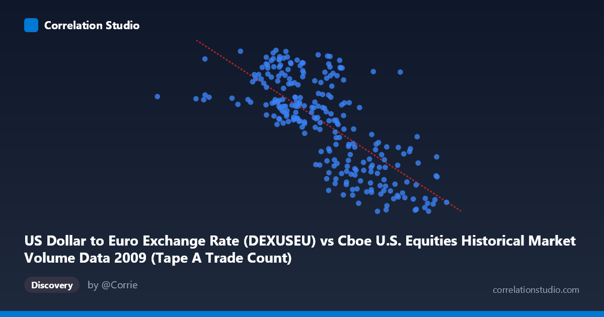
US Dollar to Euro Exchange Rate (DEXUSEU) vs Cboe U.S. Equities Historical Market Volume Data 2009 (Tape A Trade Count)
- Pearson correlation (r)
- -0.7259
- Spearman correlation
- -0.731
- p-value
- 0
- Sample size (n)
- 250
- 95% confidence interval
- -0.7797 to -0.6614
- Granger causality
- None
- Granger optimal lag
- 1
- Time coverage
- 2009-01-02 to 2009-12-31
- Recomputed on refreshed data
- 2026-10-20 (r was -0.7259)
AI analysis
Analysis: US Dollar to Euro Exchange Rate vs. Cboe Tape A Trade Count (2009)
Relationship Overview
The scatterplot reveals a moderately strong negative relationship between the US Dollar to Euro exchange rate and Cboe U.S. Equities Tape A trade counts during 2009. As the exchange rate increases (dollar strengthening relative to the euro), trade counts tend to decrease, and vice versa. The linear regression equation (y = -1.35337E-07x + 1.61487) captures this downward slope, indicating that for every unit increase in trade volume on the X-axis, the exchange rate declines by approximately 1.35 × 10⁻⁷ units — a relationship that, while statistically robust, reflects underlying macroeconomic dynamics specific to the post-financial crisis recovery period of 2009.
Correlation Strength and Statistical Framing
The correlation coefficient of r = -0.726 indicates a substantial negative association, and the R² of 0.527 means that roughly 52.7% of the variance in the Euro exchange rate is explained by variation in trade count — a meaningfully large proportion for financial time series data. The 95% confidence interval of [-0.780, -0.661] is relatively tight and entirely negative, reinforcing that the direction and magnitude of this relationship are estimated with reasonable precision given the sample of 250 paired observations drawn from a population of 3,232. The p-value of effectively zero confirms this is not a chance finding. However, the Granger causality results complicate any causal narrative: neither X→Y (F = 0.394, p = 0.531) nor Y→X (F = 1.778, p = 0.184) reaches significance at conventional thresholds, meaning that despite the strong contemporaneous correlation, neither variable reliably predicts the other in the next time period. This is a critical caveat — the relationship appears to be driven by shared temporal dynamics rather than a direct predictive mechanism in either direction.
Notable Patterns, Clusters, and Outliers
Several features stand out in the data. There is a visible cluster of high trade-count observations (roughly 1.8M–2.5M on the X-axis) that consistently correspond to lower exchange rates (~1.26–1.35), consistent with the negative trend. Conversely, lower trade counts (~800K–1.4M) tend to cluster around higher exchange rates (~1.40–1.51). A notable outlier exists at approximately (362,081, 1.44), representing an unusually low trade count with a mid-range exchange rate — potentially a holiday-shortened trading session or data anomaly. The scatter also appears somewhat heteroscedastic, with greater vertical spread at moderate trade count values, suggesting the linear model may not capture all of the distributional nuance. There is no strong evidence of a non-linear curve in the sampled points, though the moderate residual variance (47.3% unexplained) leaves room for more complex functional forms.
Confounding Factors and Interpretation Caveats
Several confounds warrant caution before interpreting this correlation substantively. 2009 was a highly anomalous year — the global financial crisis recovery, quantitative easing programs, and extraordinary market volatility all coincided, creating conditions unlikely to generalize to other periods. Both variables likely share a common driver in market stress and risk sentiment: high fear or volatility tends to simultaneously increase equity trading volume and weaken the dollar (as investors seek safe havens denominated in other currencies or exit risk assets). The dataset labels also appear potentially transposed in the axis descriptions — Tape A Trade Count is labeled on the Y-axis while the dataset descriptor calls it the exchange rate source, suggesting a possible metadata inconsistency that should be verified before drawing firm conclusions. Additionally, since these are daily time series, autocorrelation within each series may artificially inflate the apparent strength of the contemporaneous correlation.
Actionable Insights and Further Investigation
Given the strong correlation but absent Granger causality, the most productive next steps would involve investigating the common factor hypothesis — specifically, whether a latent variable such as the VIX (volatility index), Federal Reserve policy announcements, or broad risk-off sentiment simultaneously drives both series. Researchers should apply vector autoregression (VAR) with additional control variables to partial out these shared drivers. Testing this relationship across multiple years would reveal whether the 2009 pattern is structural or crisis-specific. It would also be valuable to examine lead-lag relationships at longer horizons (beyond the single lag tested here) and to verify the metadata labeling of the axes to ensure the analytical framework is correctly specified before any policy or trading conclusions are drawn.
X dataset: Cboe U.S. Equities Historical Market Volume Data 2009
Y dataset: US Dollar to Euro Exchange Rate
Part of experiment: Daily - Cboe U.S. Equities Historical Market Volume Data 2009 vs US Dollar to Euro Exchange Rate