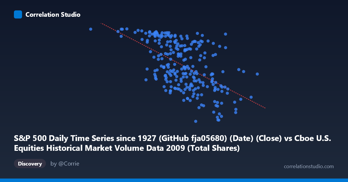
S&P 500 Daily Time Series since 1927 (GitHub fja05680) (Date) (Close) vs Cboe U.S. Equities Historical Market Volume Data 2009 (Total Shares)

Pearson correlation (r): -0.5553
Spearman correlation: -0.5511
p-value: 0
Sample size (n): 252
95% confidence interval: -0.6353 to -0.4636
Granger causality: X → Y
Granger optimal lag: 10

AI analysis

Analysis: S&P 500 Price vs. Cboe Total Shares Volume (2009)

Relationship Overview The scatterplot reveals a moderate negative relationship between the S&P 500 closing price (X-axis) and total U.S. equity shares traded on Cboe exchanges (Y-axis) throughout 2009. As the S&P 500 index level increased across the year — recovering from its March 2009 financial crisis lows — total share volume tended to decline. This is visually consistent with the linear regression equation y = -4.13×10⁻⁷x + 1261.75, meaning that for every ~2.4 million point increase in the index level, expected share volume drops by roughly 1 unit. The relationship reflects a well-documented market phenomenon: panic-driven selling and volatility during market downturns generates extremely high trading volumes, while calmer bull market rallies tend to occur on relatively lighter volume.

Correlation Strength and Statistical Significance The Pearson correlation of r = -0.5553 indicates a moderate negative association, and the R² of 0.3084 tells us that approximately 30.8% of the variance in share volume is explained by the S&P 500 price level — meaningful, but leaving nearly 70% of variability attributable to other factors. The 95% confidence interval of [-0.6353, -0.4636] is entirely negative and relatively tight, reinforcing that the negative direction is robust and not an artifact of sampling. The p-value of effectively 0 confirms the relationship is highly statistically significant across the population of N = 3,232 trading observations. Critically, the Granger causality analysis identifies a unidirectional predictive relationship: X (S&P 500 price) Granger-causes Y (share volume) at an optimal lag of 10 trading periods (F = 2.384, p = 0.011), while the reverse direction fails to reach significance (p = 0.081). This suggests that changes in index price levels have temporal predictive power over subsequent trading volume roughly two weeks later — potentially as investors reassess positioning following sustained price moves.

Notable Patterns and Outliers Several structural features are visible in the data. The point cluster at lower X values (index levels roughly 650–800, corresponding to early 2009 crisis lows) shows elevated and widely dispersed Y values, consistent with the extreme volatility and fear-driven volume surges of that period. Conversely, points at higher X values (900–1,200+, mid-to-late 2009 recovery) display lower and more tightly bunched volume figures. The point (192,269,942.50, 1126.48) stands out as a potential outlier with an unusually low X value yet high volume, and (1,212,524,830.85, 907.39) represents the highest index observation with moderate volume. There is also a visible fan-shaped heteroscedasticity — variance in Y is larger at low X values and compresses as X increases — suggesting the linear model may underfit the low-price, high-volatility regime and that a log-transformed or piecewise model could better capture the relationship.

Confounding Factors and Caveats Several important caveats temper causal interpretation. First, 2009 is a highly atypical year — it spans the tail of the worst financial crisis since the Great Depression and a dramatic V-shaped recovery, meaning both variables are simultaneously driven by a dominant third factor: macroeconomic crisis severity and investor sentiment. The correlation likely captures this shared external shock rather than a structural price-volume mechanism. Second, algorithmic and high-frequency trading volumes were accelerating in 2009 and may introduce noise into share count metrics that doesn't reflect genuine investor participation. Third, Granger causality confirms temporal precedence but does not establish economic causation — the 10-period lag relationship could be mediated by volatility indices (VIX), institutional rebalancing cycles, or options expiration calendars. Finally, using raw index level (rather than returns or volatility measures) as the X variable conflates the time trend of recovery with the price-volume dynamic.

Actionable Insights and Further Investigation Practitioners and researchers should consider several follow-up analyses. Replacing raw price with realized volatility or VIX as the independent variable would test whether it is price level or price uncertainty driving volume — a more theoretically grounded hypothesis. Segmenting the data into pre- and post-March 2009 recovery phases could reveal whether the negative correlation holds symmetrically in both crisis and recovery regimes, or whether it is asymmetric. Given the Granger result, a lagged predictive model (10-day lag) of volume from price changes could have practical utility for liquidity forecasting and trade execution timing. Additionally, log-transforming both variables would address heteroscedasticity and likely produce a more stable regression. Longer multi-year analysis spanning normal market conditions would help determine whether this 2009 relationship generalizes or is fundamentally a crisis-era artifact.

X dataset: Cboe U.S. Equities Historical Market Volume Data 2009

Y dataset: S&P 500 Daily Time Series since 1927 (GitHub fja05680) (Date)

Part of experiment: Daily - Cboe U.S. Equities Historical Market Volume Data 2009 vs S&P 500 Daily Time Series since 1927 (GitHub fja05680) (Date)