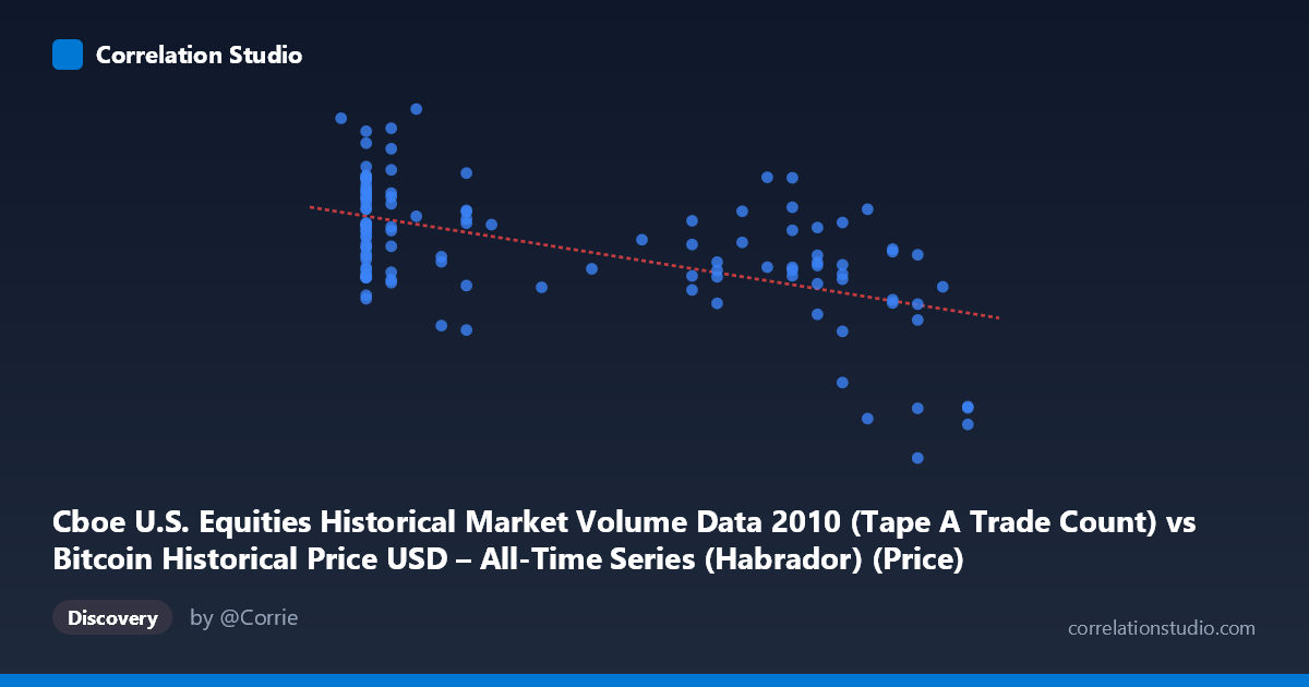
Cboe U.S. Equities Historical Market Volume Data 2010 (Tape A Trade Count) vs Bitcoin Historical Price USD – All-Time Series (Habrador) (Price)
- Pearson correlation (r)
- -0.5616
- Spearman correlation
- -0.4798
- p-value
- 0
- Sample size (n)
- 117
- 95% confidence interval
- -0.6744 to -0.4232
- Granger causality
- None
- Granger optimal lag
- 10
AI analysis
Analysis: Cboe Trade Count vs. Bitcoin Price (2010)
1. Relationship Overview
The scatterplot shows a moderate negative linear relationship between the X variable (Cboe Tape A trade counts) and Y (Bitcoin price in USD). As X increases from its minimum (~0.05) toward its maximum (~0.30), Y tends to decline from roughly 1.2–1.5M toward 500–900K. The regression line (y = -1,330,490x + 1,256,320) confirms this downward slope, though the scatter around that line is substantial, indicating the relationship is real but far from deterministic.
2. Strength, Direction, and Predictive Value
The correlation coefficient (r = -0.5616) indicates a moderate negative correlation, with r² = 0.3154 meaning only about 31.5% of the variance in Y is explained by X — the majority (68.5%) is driven by other factors entirely unaccounted for in this bivariate model. The 95% CI [-0.6744, -0.4232] is reasonably tight and excludes zero, and the p-value (4.49E-11) is highly significant, so we can be confident the negative association is not due to chance in this sample. However, statistical significance with n=117 should not be conflated with strength of practical predictive power — r² of 0.32 leaves substantial unexplained variance. Critically, the Granger causality tests (both directions non-significant, p 0.6) indicate no temporal predictive relationship in either direction at the tested lag structure. This suggests the correlation is likely a contemporaneous or spurious association (e.g., both variables trending over the same calendar period) rather than one variable causally driving or forecasting the other.
3. Notable Patterns and Outliers
Several features stand out: - Clustering at low X (~0.06–0.10): A dense cluster of points shows high variance in Y (ranging from ~800K to ~1.46M) at nearly the same X value, suggesting X alone poorly constrains Y in this region — other variables are influencing price here. - A distinct low-X, high-Y "spike" cluster: Points like (0.06, 1456720) and (0.06, 1302206) sit well above the trend line, hinting at short-term price surges independent of X. - High-X tail (~0.28–0.30): Y values compress into a lower, tighter band (489K–890K), suggesting a possible floor effect or reduced volatility at high X. - Mid-range irregularities: Points like (0.22, 1304647.53) and (0.21, 1192687.73) break the general downward trend, indicating non-linear or regime-dependent behavior rather than a clean linear decay.
4. Confounding Factors and Caveats
Since both series represent time-indexed data from 2010 (Bitcoin's genesis year) paired against Cboe equities trade counts, the negative correlation may simply reflect shared time trends — Bitcoin price was highly volatile/rising in late 2010 while equities trade volume patterns moved independently for unrelated macro reasons. This is a classic case of spurious correlation via a common time axis, especially given the non-significant Granger causality. Additionally, n=117 is a small sample relative to the stated population of 3,302, so sampling method (every-nth-point extraction) could introduce selection artifacts. There's no theoretical mechanism connecting Tape A equity trade counts to Bitcoin price in 2010 (Bitcoin markets were nascent, illiquid, and largely disconnected from mainstream equities infrastructure), which further supports treating this as coincidental rather than causal.
5. Suggestions for Further Investigation
1. Control for time directly: Include a time/trend variable in a multivariate model to see if the X-Y relationship survives after detrending both series. 2. Test stationarity: Run ADF/KPSS tests on both series — non-stationary trending series often produce spurious correlations. 3. Explore non-linear fits: The clustering pattern suggests a piecewise or log-linear relationship might fit better than a single linear model. 4. Segment by regime: Analyze low-X and high-X subgroups separately, since variance and slope appear to differ across the X range. 5. Reconsider the pairing: Given the lack of Granger causality and no plausible economic mechanism, treat this correlation as a statistical curiosity rather than an actionable signal, and prioritize investigating each variable against more directly relevant covariates (e.g., Bitcoin price vs. mining difficulty or trading volume in BTC markets).
X dataset: Bitcoin Historical Price USD – All-Time Series (Habrador)
Y dataset: Cboe U.S. Equities Historical Market Volume Data 2010
Part of experiment: Bitcoin - Bitcoin Historical Price USD – All-Time Series (Habrador) vs Cboe U.S. Equities Historical Market Volume Data 2010