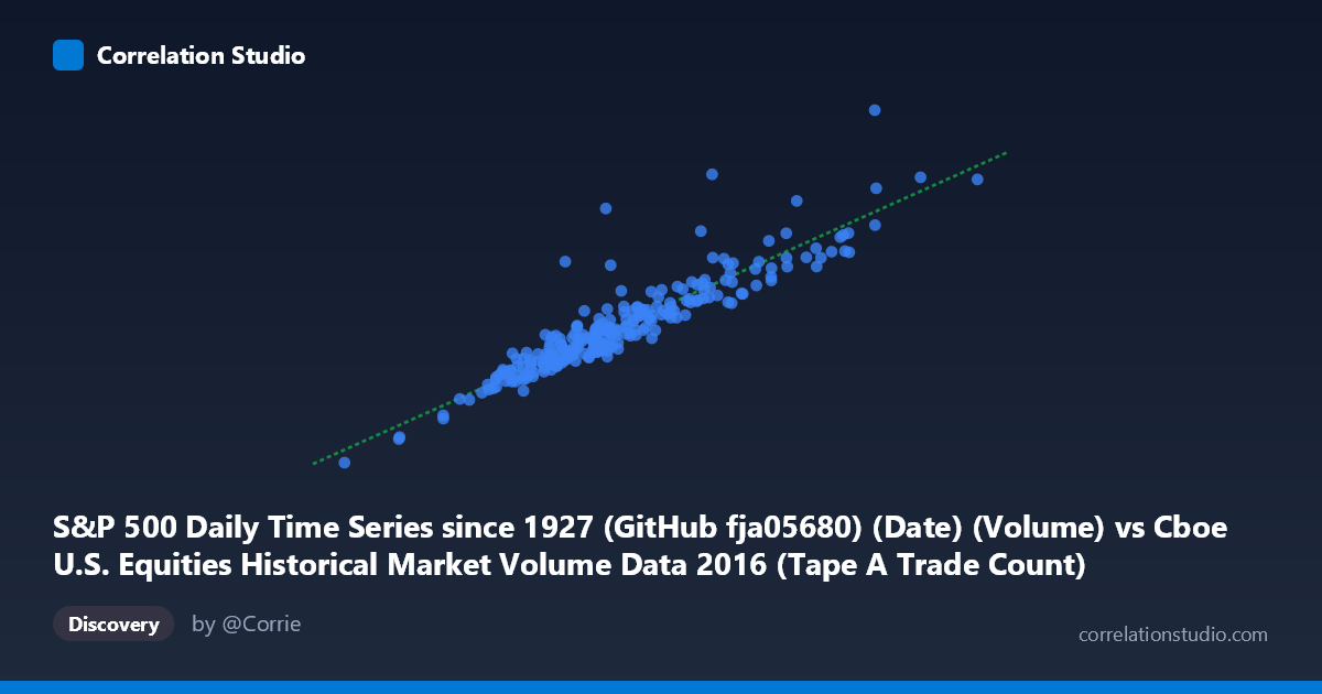
S&P 500 Daily Time Series since 1927 (GitHub fja05680) (Date) (Volume) vs Cboe U.S. Equities Historical Market Volume Data 2016 (Tape A Trade Count)
- Pearson correlation (r)
- 0.9149
- Spearman correlation
- 0.9286
- p-value
- 0
- Sample size (n)
- 252
- 95% confidence interval
- 0.8922 to 0.933
- Granger causality
- None
- Granger optimal lag
- 10
AI analysis
Analysis: S&P 500 Trading Volume vs. Cboe Tape A Trade Count (2016)
Relationship Overview The scatterplot reveals a strong, positive linear relationship between S&P 500 daily trading volume and Cboe Tape A trade count across the 2016 trading year. As daily volume increases along the X-axis (ranging from approximately 540,000 to 2.5 million), the Tape A trade count rises correspondingly along the Y-axis (spanning roughly 1.58 billion to 7.60 billion). The linear regression equation (y = 2,476.19x + 4.66×10⁸) describes this relationship well, with points clustering tightly around the regression line throughout most of the observable range, confirming that higher overall market participation is broadly and consistently reflected in Cboe's Tape A transaction counts.
Correlation Strength and Statistical Significance The correlation coefficient of r = 0.9149 indicates a very strong positive association, and the R² value of 0.8371 means that 83.7% of the variance in Tape A trade count is explained by S&P 500 volume alone — a remarkably high explanatory proportion for financial market data. The 95% confidence interval for r of [0.8922, 0.9330] is notably narrow given the sample size of n = 252, reflecting high statistical precision, and the p-value of effectively 0 leaves no doubt about the relationship's significance in the sampled period. However, the Granger causality tests complicate the narrative: neither direction (X→Y: F = 1.58, p = 0.112; Y→X: F = 1.63, p = 0.101) reaches significance at the 0.05 threshold, even at the optimal lag of 10 periods. This means that while the two series are tightly correlated contemporaneously, neither variable reliably predicts the other temporally — the relationship is synchronous rather than leading/lagging, suggesting both are driven by common underlying forces rather than one causing the other.
Patterns, Clusters, and Outliers The bulk of observations cluster densely in the mid-range (X: ~1.1M–1.6M; Y: ~3.1B–4.5B), consistent with typical 2016 trading conditions. Several notable high-volume outliers appear in the upper-right quadrant — points exceeding X = 1.8M and Y = 4.7B — which likely correspond to identifiable market events such as the U.S. presidential election (November 2016) or Brexit-related volatility spillovers earlier in the year. A handful of low-volume points in the lower-left (X < 900,000; Y < 2.7B) may correspond to holiday-shortened sessions or unusually quiet summer days. Critically, even these extreme points appear to respect the linear trend rather than deviating markedly from it, reinforcing the robustness of the relationship across varied market conditions. No strong non-linear curvature is apparent, though slight heteroscedasticity may exist at higher volume levels where scatter appears to widen modestly.
Confounding Factors and Caveats Several important caveats temper interpretation. First, both variables are likely co-driven by the same latent factor: aggregate market activity. High-volatility or high-sentiment days naturally inflate both overall S&P 500 volume and Tape A trade counts simultaneously, making the high correlation partially tautological. Second, the dataset covers only a single calendar year (2016), a period with specific macroeconomic characteristics; the relationship may not generalize to other market regimes (e.g., post-COVID volumes, algorithmic trading shifts). Third, Tape A specifically covers NYSE-listed securities, while the S&P 500 volume figure aggregates across multiple venues, introducing definitional asymmetry that could distort the relationship if routing behavior changes. Finally, the population size of N = 3,622 versus the paired sample of n = 252 warrants attention — the sampling methodology should be verified to ensure representativeness.
Actionable Insights and Further Investigation Practitioners could explore whether this relationship holds across multiple years to test its stability as a real-time proxy model — if Tape A trade count reliably tracks total S&P volume, either could serve as a redundant signal for market activity monitoring. The absence of Granger causality suggests that intraday or higher-frequency data might reveal leading/lagging dynamics invisible at the daily aggregation level; investigating tick-level or hourly data could be valuable. It would also be worthwhile to decompose the outlier events — confirming whether the upper-right cluster maps to November 8–9 (election) and June 24 (Brexit) would validate the model's behavior under stress. Finally, extending this analysis to other Tape designations (Tape B for NYSE-American, Tape C for Nasdaq) would determine whether the correlation is specific to NYSE-listed securities or represents a market-wide phenomenon.
X dataset: Cboe U.S. Equities Historical Market Volume Data 2016
Y dataset: S&P 500 Daily Time Series since 1927 (GitHub fja05680) (Date)
Part of experiment: Daily - Cboe U.S. Equities Historical Market Volume Data 2016 vs S&P 500 Daily Time Series since 1927 (GitHub fja05680) (Date)