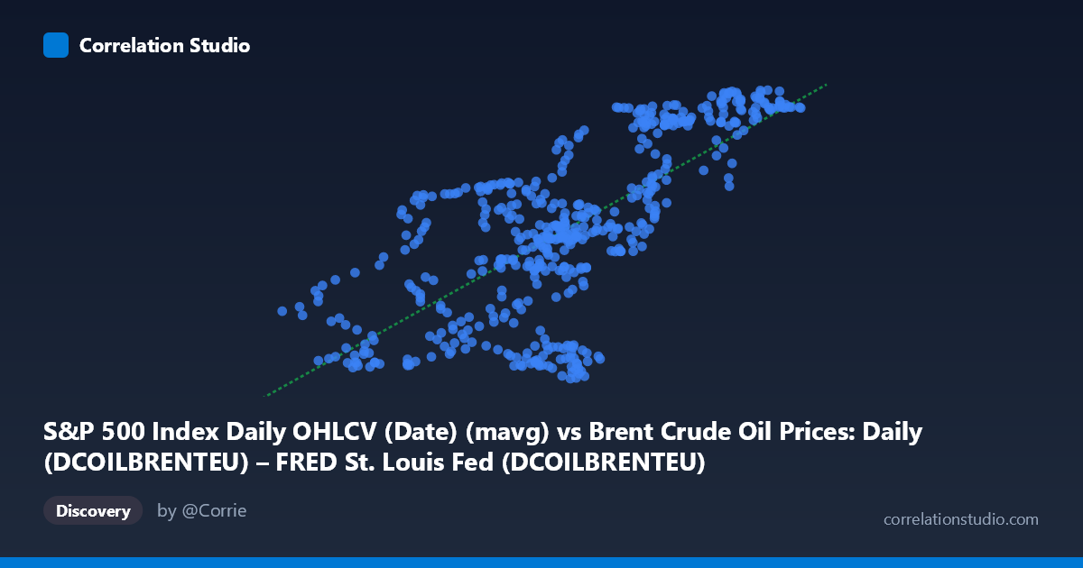
S&P 500 Index Daily OHLCV (Date) (mavg) vs Brent Crude Oil Prices: Daily (DCOILBRENTEU) – FRED St. Louis Fed (DCOILBRENTEU)
- Pearson correlation (r)
- 0.7175
- Spearman correlation
- 0.6961
- p-value
- 0
- Sample size (n)
- 504
- 95% confidence interval
- 0.6723 to 0.7574
- Granger causality
- None
- Granger optimal lag
- 1
AI analysis
Analysis: S&P 500 Moving Average vs. Brent Crude Oil Prices (2015–2017)
1. Overall Relationship The scatterplot reveals a positive, moderately strong linear relationship between the S&P 500 Index moving average and Brent Crude Oil prices over the two-year period from February 2015 to February 2017. As the S&P 500 moving average rises from roughly 26 to 66, Brent crude prices tend to climb from approximately 94 to 130 USD per barrel. The fitted regression line (y = 0.887x + 69.91) captures this upward trend reasonably well, though considerable scatter around the line suggests meaningful unexplained variation. Visually, the data forms an elongated cloud oriented from lower-left to upper-right, consistent with a positive association, but with notable vertical spread at nearly every level of X.
2. Correlation Strength, Statistical Significance, and Causal Direction The Pearson correlation of r = 0.7175 indicates a moderately strong positive association, and with r² = 0.5148, approximately 51.5% of the variance in Brent crude prices is explained by the S&P 500 moving average — meaning nearly half the variance remains unexplained by this relationship alone. The 95% confidence interval of [0.6723, 0.7574] is relatively tight and sits entirely above zero, and the p-value of effectively 0 confirms this correlation is highly statistically significant given n = 504 paired observations. However, the Granger causality results are particularly important here: neither direction shows significant predictive power (X→Y: F = 0.1981, p = 0.656; Y→X: F = 0.1068, p = 0.744). This means that neither variable meaningfully predicts the other in a temporal, lead-lag sense — the correlation reflects co-movement rather than directional predictive flow, strongly cautioning against any causal interpretation.
3. Notable Patterns, Clusters, and Outliers Several structural features are visible in the sample points. There appear to be two loose clusters: one concentrated in the mid-range (X ≈ 43–55, Y ≈ 105–120) representing the bulk of observations, and another at the upper-right extreme (X ≈ 61–66, Y ≈ 127–130), likely corresponding to the market recovery period in late 2016 to early 2017. Conversely, lower-left points (X ≈ 29–37, Y ≈ 95–105) correspond to the period of oil price depression in early-to-mid 2015. A few potential outliers stand out — notably points like (50.73, 96.49), (48.81, 95.18), and (46.72, 95.62) where S&P 500 values are near the mean but oil prices are unusually low, suggesting periods where the two assets diverged. Similarly, (37.66, 116.67) and (35.26, 114.42) show low S&P values paired with relatively high oil prices, hinting at non-linear or regime-dependent behavior at the tails.
4. Confounding Factors and Caveats Several important caveats apply. First, both variables are time series with strong trend components, and much of the observed correlation may reflect shared macroeconomic trends during 2015–2017 rather than any fundamental financial link — this is a textbook case where spurious correlation via common trending is plausible. The use of a moving average for the S&P 500 X-axis further smooths short-term volatility and may artificially inflate the correlation by reducing noise asymmetrically. Second, the note that the axis labels appear swapped in the dataset metadata (S&P 500 mavg is on X but drawn from the Brent dataset, and vice versa) introduces interpretive ambiguity and warrants data pipeline verification. Third, omitted variables such as USD strength, global demand shocks, OPEC production decisions, and broad risk appetite (VIX) all influence both series simultaneously, making any bivariate interpretation incomplete.
5. Actionable Insights and Further Investigation Given the absence of Granger causality, practitioners should avoid using this relationship for trading signals or directional forecasting in either direction. Instead, the co-movement likely reflects a shared sensitivity to global macroeconomic risk sentiment, which would be worth modeling explicitly — for instance, by including a risk appetite proxy or USD index as a control variable in a multivariate regression. A rolling correlation analysis across sub-periods would reveal whether this r ≈ 0.72 relationship is stable or regime-dependent, as oil-equity correlations are known to shift dramatically around supply shocks or recessions. Additionally, detrending both series (via differencing or removing a common trend component) before computing correlation would better isolate genuine co-movement from spurious trend-driven association. Finally, verifying and correcting the apparent axis/dataset label mismatch in the metadata should be the immediate first step before drawing any further conclusions.
X dataset: Brent Crude Oil Prices: Daily (DCOILBRENTEU) – FRED St. Louis Fed
Y dataset: S&P 500 Index Daily OHLCV (Date)
Part of experiment: Daily - Brent Crude Oil Prices: Daily (DCOILBRENTEU) – FRED St. Louis Fed vs S&P 500 Index Daily OHLCV (Date)