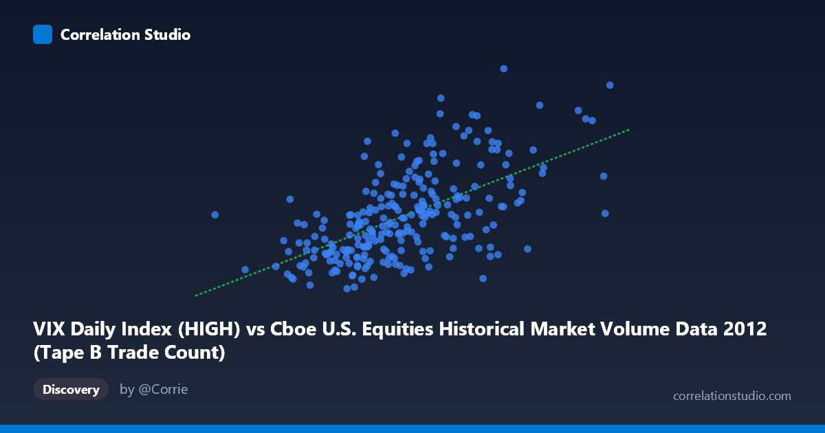
VIX Daily Index (HIGH) vs Cboe U.S. Equities Historical Market Volume Data 2012 (Tape B Trade Count)
- Pearson correlation (r)
- 0.5888
- Spearman correlation
- 0.5966
- p-value
- 0
- Sample size (n)
- 250
- 95% confidence interval
- 0.5013 to 0.6643
- Granger causality
- None
- Granger optimal lag
- 1
- Time coverage
- 2012-01-03 to 2012-12-31
- Recomputed on refreshed data
- 2026-10-09 (r was 0.5888)
AI analysis
Scatterplot Analysis: VIX Daily Index (HIGH) vs. Tape B Trade Count
Relationship Overview
The scatterplot reveals a moderate positive relationship between the VIX Daily Index High values and the Cboe U.S. Equities Tape B Trade Count across the 2012 trading year. As the VIX High increases — reflecting elevated market volatility expectations — the Tape B trade count tends to rise correspondingly. This is intuitively consistent with market microstructure theory: heightened volatility environments typically stimulate greater trading activity as participants react to uncertainty, rebalance positions, or execute hedges. The linear regression equation (y = 4.00301E-05x + 11.5592) confirms a positive slope, meaning each unit increase in VIX High is associated with a small but meaningful uptick in trade count. However, the scatter around the regression line is visually substantial, suggesting the relationship is real but far from deterministic.
Correlation Strength and Statistical Significance
The Pearson correlation of r = 0.5888 indicates a moderate positive association, but the more informative statistic is r² = 0.3467, meaning that VIX High explains only approximately 34.7% of the variance in Tape B Trade Count. The remaining ~65% of variability is attributable to factors outside this model. The 95% confidence interval of [0.5013, 0.6643] is relatively tight given the sample size of n = 250 drawn from a population of N = 3,750, and the p-value of effectively zero confirms that this correlation is highly statistically significant — almost certainly not a chance finding. That said, statistical significance should not be conflated with practical or causal significance, especially given that one-third of variance explained leaves considerable unexplained noise. The Granger causality results are particularly important here: neither direction (X→Y: F = 1.75, p = 0.187; Y→X: F = 0.10, p = 0.758) reaches statistical significance at conventional thresholds. This means that past values of VIX High do not reliably predict future Tape B Trade Counts, and vice versa — the contemporaneous correlation does not translate into temporal predictive power, a critical caveat for any trading or forecasting application.
Notable Patterns, Clusters, and Outliers
Several features stand out in the sample data. There is a discernible concentration of observations in the X range of roughly 130,000–220,000 (VIX High values), with trade counts clustering between approximately 15 and 21 — this central mass forms the core of the positive trend. However, there are notable outliers and high-leverage points: for instance, the observation at approximately (295,121, 18.75) sits far to the right on the X-axis yet has a relatively moderate trade count, pulling against the positive trend. Conversely, points like (197,126, 24.93) and (170,460, 23.73) show high trade counts at moderate VIX levels, suggesting some episodes of elevated trading activity that are not VIX-driven. The data also hints at heteroscedasticity — variance in trade counts appears to widen at higher VIX levels — and there may be non-linear saturation effects where very high VIX values do not continue to drive proportional increases in trading volume.
Confounding Factors and Interpretive Caveats
Several important caveats temper interpretation. Dataset labeling warrants careful scrutiny: the axes as described show X as "VIX Daily Index HIGH" sourced from the Cboe Market Volume dataset, while Y is "Tape B Trade Count" sourced from the VIX Daily Index dataset — this appears to reflect a cross-dataset pairing that may introduce structural mismatches in how variables are recorded or aggregated. Additionally, 2012 was a specific macro regime (post-financial crisis recovery, European debt concerns, U.S. election year) that may not generalize to other periods. Tape B specifically covers NYSE American (AMEX) and regional exchange securities, which may respond to volatility differently than broader market segments. Seasonality, day-of-week effects, and macro event clustering (earnings seasons, Fed announcements) could simultaneously elevate both VIX and trade counts, creating spurious correlation without a direct causal mechanism. The absence of Granger causality further underscores that common drivers — rather than a direct link — likely explain the observed correlation.
Actionable Insights and Further Investigation
Despite the absence of Granger causality, the moderate contemporaneous correlation (r ≈ 0.59) is strong enough to be practically informative in certain contexts. Exchange operators and market makers could use VIX regime classification (low/medium/high) as a rough signal for anticipated Tape B volume load planning. For researchers, the next logical steps include: (1) testing non-linear models (e.g., log-log transformation or polynomial regression) given potential heteroscedasticity and saturation at extreme VIX values; (2) expanding the time window beyond 2012 to assess whether the relationship is stable across different volatility regimes; (3) including additional covariates such as overall market volume (Tape A/C), S&P 500 returns, and macroeconomic event dummies to better isolate the VIX effect; and (4) investigating the outlier observations — particularly the high-X/moderate-Y and moderate-X/high-Y points — to determine whether they represent specific market events that could enrich the explanatory model.
X dataset: Cboe U.S. Equities Historical Market Volume Data 2012
Y dataset: VIX Daily Index
Part of experiment: Daily - Cboe U.S. Equities Historical Market Volume Data 2012 vs VIX Daily Index