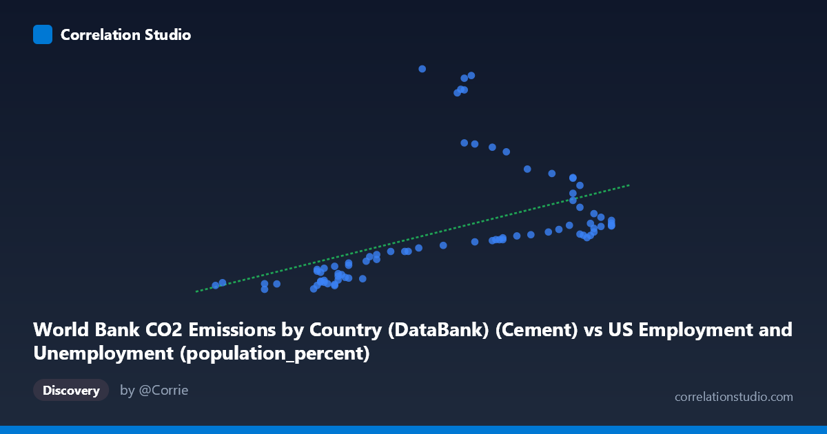
World Bank CO2 Emissions by Country (DataBank) (Cement) vs US Employment and Unemployment (population_percent)
- Pearson correlation (r)
- 0.5021
- Spearman correlation
- 0.7753
- p-value
- 0.000002
- Sample size (n)
- 80
- 95% confidence interval
- 0.3174 to 0.6501
- Granger causality
- None
- Granger optimal lag
- 10
AI analysis
Analysis of World Bank CO2 Cement Emissions vs. US Employment/Unemployment Population Percent
1. What the Visualization Reveals
The scatterplot displays a moderate positive relationship between cement-related CO2 emissions (X-axis) and a US employment/unemployment population percentage metric (Y-axis), spanning data from 1941 to 2020. The linear regression line (y = 98.81x − 5406.53) slopes upward across the X range of roughly 55.8 to 67.1, with Y values spanning an enormous range from approximately 79 to 2,609. Critically, the plot reveals substantial vertical dispersion at nearly every X value — particularly in the mid-range (X ≈ 62–64), where Y values scatter from around 500 to over 2,500 — indicating that the linear model captures only a fraction of the observed variability.
2. Correlation Strength, Direction, and Statistical Framing
The Pearson correlation of r = 0.5021 indicates a moderate positive association, but the coefficient of determination r² = 0.2521 tells a more sobering story: only 25.2% of the variance in Y is explained by X, leaving nearly three-quarters of the variation unexplained by this linear relationship. The 95% confidence interval for r of [0.317, 0.650] is notably wide, reflecting meaningful uncertainty in the true population correlation despite statistical significance. The p-value of 2.08×10⁻⁶ confirms the association is highly unlikely to be due to chance alone given n = 80 paired observations, so the signal is real — but modest. Granger causality testing finds no significant predictive directionality in either direction (X→Y: F = 0.52, p = 0.87; Y→X: F = 1.99, p = 0.055), meaning neither variable reliably temporally precedes or predicts the other in a lagged framework, effectively ruling out a straightforward causal narrative even at the optimal lag of 10 periods.
3. Notable Patterns, Clusters, and Outliers
Several features demand attention. There is a high-density cluster of low Y values (roughly 78–500) concentrated at the lower end of X (55.8–61.5), suggesting a somewhat different behavioral regime at lower cement emission levels. A striking cluster of extreme Y outliers appears near X ≈ 61.7–63.2, where values reach 2,333–2,609 — points like (62.70, 2333.75), (62.90, 2501.79), (63.10, 2532.94), and (61.70, 2608.93) sit dramatically above the regression line and likely exert disproportionate leverage on the correlation. The Spearman ρ exceeding Pearson r is a key diagnostic flag, confirming that a non-linear relationship (polynomial or logarithmic) would likely fit the data better than the current linear model. The distribution appears to show a possible fan or heteroscedastic shape, with variance in Y increasing as X increases.
4. Confounding Factors and Interpretive Caveats
The pairing of cement CO2 emissions (a global industrial metric) with a US employment/unemployment population percentage is conceptually indirect, and the observed correlation is almost certainly mediated by a shared underlying driver: long-run economic growth and industrialization. Both variables tend to increase over time across this 80-year span, making temporal autocorrelation and spurious correlation via secular trends a primary concern. The absence of Granger causality supports this interpretation — they are likely co-moving with the global or US economy rather than causally linked. The high-Y outlier cluster may correspond to specific historical periods (e.g., post-WWII economic expansion or specific labor force participation shifts) that are entirely unrelated to cement production. Dataset labeling also warrants scrutiny: the axis labels suggest a possible dataset join mismatch, where "Cement" emissions from a global dataset are being compared to a US-specific labor metric, creating an ecological inference problem.
5. Actionable Insights and Further Investigation
Given the non-linear signal identified by Spearman ρ, the first priority should be fitting polynomial or logarithmic regression models and comparing them via AIC/BIC to the linear model. Investigators should partial out the time trend (detrend both series) to test whether any correlation persists after removing shared secular growth, as this would distinguish genuine covariation from spurious trend alignment. The outlier cluster near X = 62–63.2 warrants individual-year identification to determine whether they represent a specific economic episode or data quality issues. Expanding the Granger causality analysis with different lag structures or applying cointegration tests (e.g., Engle-Granger) would better assess whether a long-run equilibrium relationship exists. Finally, if the research goal is meaningful, replacing the global cement emissions variable with US-specific cement or construction industry emissions would create a more theoretically coherent pairing with the labor market variable.
X dataset: US Employment and Unemployment
Y dataset: World Bank CO2 Emissions by Country (DataBank)
Part of experiment: Yearly - US Employment and Unemployment vs World Bank CO2 Emissions by Country (DataBank)