S&P 500 Daily Time Series since 1927 (GitHub fja05680) (Date) (Volume) vs Cboe U.S. Equities Historical Market Volume Data 2013 (Tape B Notional)
- Pearson correlation (r)
- 0.6736
- Spearman correlation
- 0.607
- p-value
- 0
- Sample size (n)
- 252
- 95% confidence interval
- 0.5999 to 0.7359
- Granger causality
- None
- Granger optimal lag
- 10
AI analysis
Analysis: S&P 500 Trading Volume vs. Tape B Notional Value (2013)
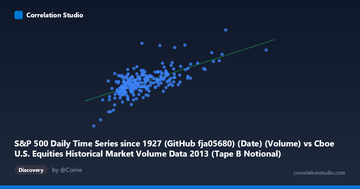
Relationship Overview The scatterplot reveals a moderate positive relationship between S&P 500 daily trading volume (X-axis, measured in shares) and Tape B notional value (Y-axis, measured in dollars) across 252 trading days in 2013. As daily trading volume increases, Tape B notional value tends to rise correspondingly, which is economically intuitive — higher overall market activity generally lifts notional dollar values traded across exchange tapes. The linear regression equation (y = 0.348x + 2.008B) suggests that for every additional unit of volume, Tape B notional value increases by approximately $0.35, anchored to a substantial baseline of ~$2 billion, reflecting the persistent dollar value of smaller-cap and regional exchange activity even on low-volume days.
Correlation Strength and Statistical Significance The correlation of r = 0.674 indicates a moderate-to-strong positive association, but the more practically meaningful figure is r² = 0.454 — meaning only 45.4% of the variance in Tape B notional value is explained by total market volume. Roughly 54.6% of variance remains unexplained, pointing to substantial independent drivers of Tape B activity. The 95% confidence interval of [0.600, 0.736] is relatively tight and excludes zero, and the p-value of effectively 0 confirms the correlation is highly statistically significant at any conventional threshold, ruling out chance as an explanation. However, the Granger causality results are notable and sobering: neither direction (X→Y nor Y→X) achieves significance (F = 0.754, p = 0.673 and F = 0.595, p = 0.818 respectively), meaning that past values of total volume do not reliably predict future Tape B notional values, and vice versa. The relationship is contemporaneous rather than predictively directional — they move together but neither leads the other temporally.
Patterns, Clusters, and Outliers The scatterplot exhibits a clear but dispersed positive trend, with notable heteroscedasticity — the spread of Y values fans outward as X increases, suggesting that high-volume days produce more variable Tape B outcomes than low-volume days. Several outliers are visible at the upper right of the distribution, most strikingly points near X = 6.56B, 7.30B, and 9.22B (well beyond the bulk of data clustered between 2.5B–5.5B), which correspond to unusually high-volume days likely tied to specific market events (index rebalancing, options expiration, macro announcements). A dense core cluster exists around X ≈ 3.0B–4.5B and Y ≈ 3.0B–3.8B, representing typical trading days. There also appear to be low-end outliers where volume is modest (~2.4B–2.6B) but Tape B notional values are disproportionately low (~1.97B–2.05B), suggesting quieter holiday-adjacent or summer trading sessions.
Confounding Factors and Caveats Several important caveats apply. First, Tape B covers NYSE American (AMEX) and regional exchange securities, which have distinct characteristics from the broader S&P 500 universe — their notional values are influenced by mid- and small-cap price levels, sector composition, and exchange-specific market-making dynamics independent of overall market volume. Second, price levels matter enormously for notional value: a high-volume day in a declining market could produce lower notional values than a moderate-volume day with elevated prices, introducing price-level confounding. Third, seasonality within 2013 (e.g., low summer/holiday volumes vs. high year-end activity) may create spurious clustering that inflates the observed correlation. Fourth, since this covers only a single calendar year (252 points), the relationship may not generalize across different volatility regimes or market cycles.
Actionable Insights and Further Investigation Practitioners should not use total volume as a predictive signal for Tape B notional value given the failed Granger causality tests — the relationship is concurrent, not leading. To improve the explanatory model, analysts should incorporate price-level variables (e.g., S&P 500 index level, VIX) and Tape B-specific volume as covariates, which could substantially increase R² beyond the current 45.4%. It would be worthwhile to examine the outlier high-volume days individually to determine whether they represent systematic event types (quadruple witching, FOMC days) that could be modeled separately. Extending this analysis across multiple years would clarify whether the 2013 correlation is regime-specific or structural. Finally, a segmented regression or quantile regression approach could better capture the heteroscedastic behavior observed at the upper tail of the volume distribution.
X dataset: Cboe U.S. Equities Historical Market Volume Data 2013
Y dataset: S&P 500 Daily Time Series since 1927 (GitHub fja05680) (Date)
Part of experiment: Daily - Cboe U.S. Equities Historical Market Volume Data 2013 vs S&P 500 Daily Time Series since 1927 (GitHub fja05680) (Date)