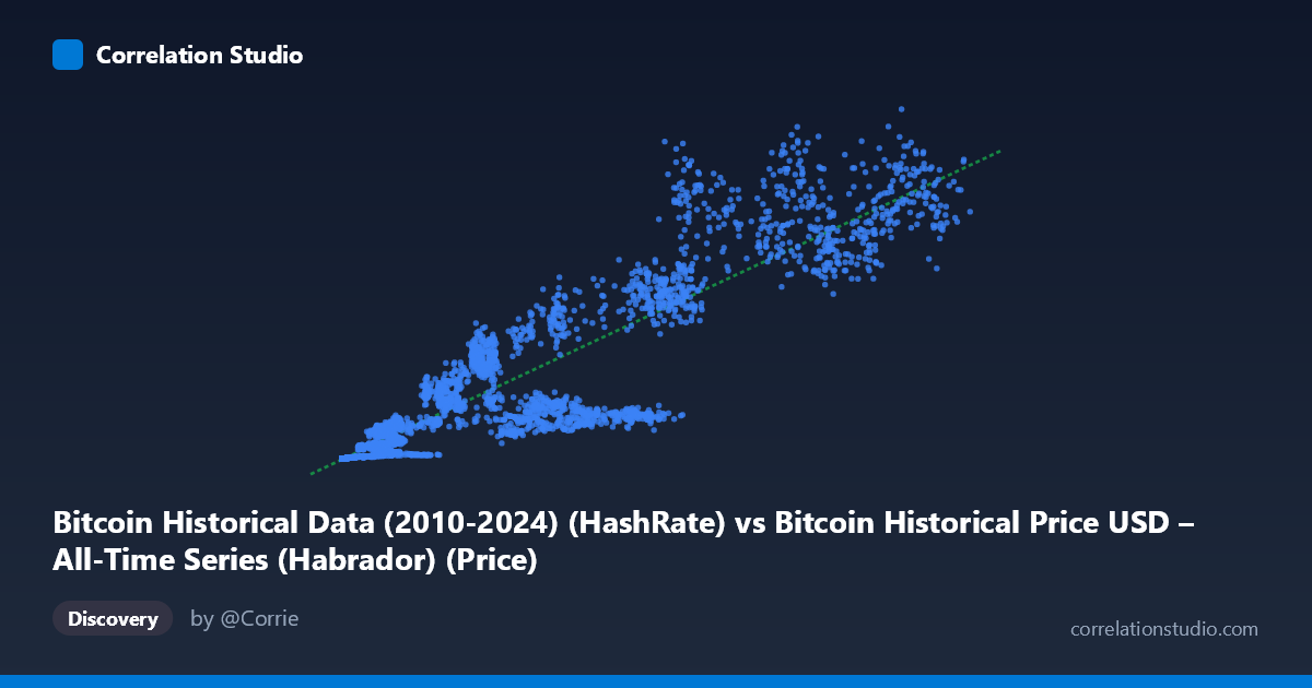
Bitcoin Historical Data (2010-2024) (HashRate) vs Bitcoin Historical Price USD – All-Time Series (Habrador) (Price)
- Pearson correlation (r)
- 0.9262
- Spearman correlation
- 0.9715
- p-value
- 0
- Sample size (n)
- 5764
- 95% confidence interval
- 0.9224 to 0.9298
- Granger causality
- None
- Granger optimal lag
- 10
- Time coverage
- 2010-07-18 to 2026-04-28
AI analysis
Analysis: Bitcoin Hash Rate vs. Price
1. What the Visualization Reveals
The scatterplot shows a strong, positive, non-linear relationship between Bitcoin's network hash rate (X) and its USD price (Y). Points near the origin (low hash rate, low price) are densely clustered, while higher hash rate values spread into a wide range of prices — suggesting the relationship, while strongly monotonic, is not strictly linear. This is consistent with Bitcoin's exponential growth trajectory on both dimensions across its history, with hash rate and price both increasing by orders of magnitude from 2010 to 2024.
2. Strength, Direction, and Statistical Interpretation
The correlation coefficient (r = 0.926) indicates a very strong positive linear association, with r² = 0.858 meaning hash rate statistically "explains" about 86% of the variance in price under a linear model. The tight confidence interval [0.922, 0.930] and p-value of effectively 0 confirm this relationship is highly unlikely to be due to chance, especially given the large sample size (n = 5,764).
However, the Granger causality results are critical for interpretation: neither variable significantly predicts the other in a temporal, lead-lag sense (X→Y: p = 0.785; Y→X: p = 0.906). This means that despite the strong contemporaneous correlation, hash rate does not systematically precede price movements (or vice versa) in a way that would support forecasting. Practically, this suggests both variables are likely driven by a shared underlying trend (e.g., overall market growth, adoption, mining profitability incentives) rather than one directly causing the other in a lagged, exploitable manner.
3. Notable Patterns and Features
The data reveals a classic "hockey stick" pattern typical of exponentially growing time series: a dense cluster of small values (early Bitcoin era, X < 1000, Y < $10M) followed by a widening, fan-like spread at higher hash rates. Notably, at similar hash rate levels (e.g., ~50,000-65,000), price varies substantially (from ~$150M to over $650M in the sample), indicating that price volatility (bull/bear cycles) occurs somewhat independently of gradual hash rate growth. This is expected — miners add hardware based on long-term profitability expectations, while price responds to short-term speculation, news, and macro sentiment, creating "slack" in the relationship at any given time.
4. Confounding Factors and Caveats
The most significant caveat is that both variables are dominated by a shared time trend — as calendar time progresses, both hash rate and price tend to rise due to network maturation and broader crypto adoption. This makes the strong r² potentially a "spurious" trend correlation rather than genuine causal linkage; the Granger test result reinforces this concern. Additionally, hash rate is arguably a lagging indicator of price (miners invest in hardware in response to past profitability), yet the Granger test doesn't detect this either, possibly due to nonlinearities, regime changes (halvings), or the 10-period lag structure not capturing the true dynamics. The linear regression (y = 8817x − 3.33M) is a poor global fit given the visible curvature — a log-log or exponential model would likely fit much better.
5. Suggestions for Further Investigation
1. Detrend or difference both series (e.g., % change, log returns) before re-running correlation/Granger tests to control for the shared exponential trend and test for genuine short-term co-movement. 2. Fit a log-log regression (log(Price) ~ log(HashRate)) given the clear exponential/power-law shape, which should substantially improve model fit and interpretability. 3. Segment by halving cycles (2012, 2016, 2020, 2024) to check if the price-hashrate relationship is stable across market regimes or shifts structurally. 4. Investigate confounders like active addresses, transaction volume, or macro liquidity conditions as potential common drivers of both series.
X dataset: Bitcoin Historical Price USD – All-Time Series (Habrador)
Y dataset: Bitcoin Historical Data (2010-2024)
Part of experiment: Bitcoin - Bitcoin Historical Price USD – All-Time Series (Habrador) vs Bitcoin Historical Data (2010-2024)