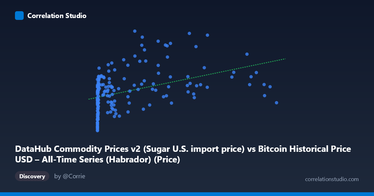
DataHub Commodity Prices v2 (Sugar U.S. import price) vs Bitcoin Historical Price USD – All-Time Series (Habrador) (Price)
- Pearson correlation (r)
- 0.4184
- Spearman correlation
- 0.5612
- p-value
- 0
- Sample size (n)
- 182
- 95% confidence interval
- 0.2906 to 0.5315
- Granger causality
- None
- Granger optimal lag
- 1
- Time coverage
- 2010-08-01 to 2025-09-01
- Recomputed on refreshed data
- 2026-10-24 (r was 0.4184)
AI analysis
Analysis: Bitcoin Price vs. Sugar Import Price
1. Overview of the Relationship
The scatterplot shows a modest positive association between Bitcoin's historical USD price (X-axis) and the U.S. sugar import price (Y-axis, likely mislabeled/swapped given the column descriptions). The data is heavily right-skewed on the X-axis — Bitcoin prices span nearly six orders of magnitude (0.06 to 113,500), with the bulk of observations clustered below 50,000 and a long tail of high-price points. This skew means the relationship is dominated by a relatively small number of high-Bitcoin-price observations, while the majority of points sit in a compressed region near the origin.
2. Strength, Direction, and Statistical Confidence
The Pearson correlation (r = 0.418) indicates a weak-to-moderate positive linear relationship, with r² = 0.175 meaning only about 17.5% of the variance in sugar prices is explained by Bitcoin price levels — leaving over 80% unexplained by this simple linear model. The 95% CI [0.29, 0.53] is reasonably tight and excludes zero, and the p-value (4.2×10⁻⁹) confirms this correlation is statistically significant and not due to chance. However, statistical significance here reflects the correlation's reliability, not its practical strength — this is a weak relationship suitable for exploratory noting, not predictive modeling. Critically, the Granger causality tests show no significant predictive direction in either direction (X→Y: p=0.66; Y→X: p=0.27), meaning neither variable's past values help forecast the other's future values in this time series. This strongly suggests the correlation is either coincidental, driven by a shared external trend (e.g., both rising over the 2010-2025 period due to inflation/time), or an artifact of non-stationarity rather than a genuine causal or leading/lagging relationship.
3. Notable Patterns and Outliers
Several features stand out: (a) a cluster of low-X, low-Y points (X < 50, Y ≈ 4.2–7.3) representing Bitcoin's early near-zero price era; (b) increasing scatter/variance in Y as X grows, suggesting heteroscedasticity; (c) some high-Y outliers (e.g., Y 10) appearing at moderate X values (23,000–46,000) rather than at the extreme high end, breaking a clean monotonic pattern; (d) the extreme X-tail (90,000) doesn't show correspondingly extreme Y values, suggesting the relationship flattens or saturates at high Bitcoin prices. The note that Spearman ρ exceeds Pearson r reinforces this — a logarithmic or monotonic-but-nonlinear relationship (e.g., log(X) vs Y) likely fits better than a straight line, consistent with the massive scale range of X.
4. Confounding Factors and Caveats
The most important caveat is that both series are long-run time trends — Bitcoin's price grew ~6 orders of magnitude from 2010–2025, and commodity prices (including sugar) also drifted upward over this period due to general inflation, currency debasement, and macroeconomic cycles. This is a classic case of spurious correlation via shared temporal trend: two unrelated non-stationary series will often show significant Pearson correlation simply because both increase over time, without any causal linkage. The lack of Granger causality supports this interpretation. Additionally, mismatched sampling frequency (Bitcoin trades continuously; sugar prices are monthly) and potential label-swapping in the axis descriptions (the dataset naming appears crossed) should be verified before drawing conclusions.
5. Recommendations for Further Investigation
Before treating this as a meaningful relationship: (1) detrend both series (e.g., use log returns or differences rather than levels) and re-test correlation/Granger causality — this is the standard fix for spurious time-trend correlations; (2) fit a log-linear model (log(X) vs Y) given the Spearman/Pearson discrepancy and extreme X-skew; (3) verify axis/column labeling given the apparent dataset-description mismatch; (4) if genuine interest exists in Bitcoin-commodity linkages, test against a common macro driver (USD index, inflation rate, M2 money supply) as a control variable to rule out confounding. Given r²=17.5% and no Granger causality, this correlation should not be used for forecasting or trading strategies in its current form.
X dataset: Bitcoin Historical Price USD – All-Time Series (Habrador)
Y dataset: DataHub Commodity Prices v2
Part of experiment: Bitcoin - Bitcoin Historical Price USD – All-Time Series (Habrador) vs DataHub Commodity Prices v2