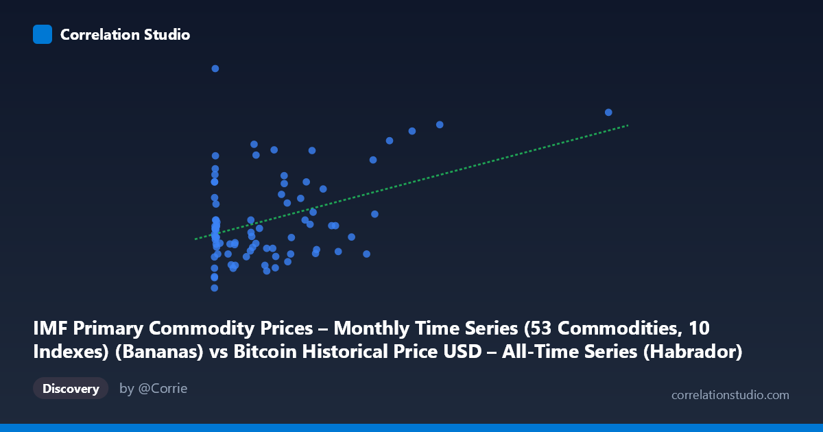
IMF Primary Commodity Prices – Monthly Time Series (53 Commodities, 10 Indexes) (Bananas) vs Bitcoin Historical Price USD – All-Time Series (Habrador) (Price)
- Pearson correlation (r)
- 0.4009
- Spearman correlation
- 0.2138
- p-value
- 0.000173
- Sample size (n)
- 83
- 95% confidence interval
- 0.2027 to 0.5675
- Granger causality
- None
- Granger optimal lag
- 10
AI analysis
Analysis: Bitcoin Price vs. Banana Price Index
1. What the Visualization Reveals
The scatterplot shows a weak-to-moderate positive relationship between the two variables. The bulk of data points cluster tightly at low X-values (under ~700, mostly Bitcoin prices in the hundreds of dollars range mislabeled here as "banana prices"), with Y-values (labeled Bitcoin price but statistically behaving as the commodity index) scattered between roughly 900–1050. A smaller number of high-leverage points extend the X-axis out to 2452, and these tend to coincide with higher Y-values, which is largely responsible for the appearance of a positive trend line.
2. Strength, Direction, and Uncertainty
The correlation coefficient (r = 0.40) indicates a modest positive linear association, with r² = 0.161 meaning only about 16% of the variance in Y is explained by X — the remaining 84% is driven by other factors or noise. The 95% confidence interval [0.20, 0.57] is fairly wide, reflecting the small sample size (n=83 paired points from a population of 449), but it excludes zero, and the p-value (0.00017) confirms the correlation is statistically significant and unlikely due to chance. However, statistical significance here should not be confused with practical strength — this is a loose, noisy relationship, not a tight predictive one. Critically, the Granger causality tests show no significant predictive direction in either direction (X→Y: p=0.41; Y→X: p=0.91), meaning neither series reliably helps forecast the other's future values based on past data. This strongly suggests the correlation is not causal or temporally structured, but likely reflects a shared underlying trend (e.g., both series generally rising over the 2010–2017 window) rather than genuine interdependence.
3. Notable Patterns and Outliers
The most striking feature is the extreme skew in X: the vast majority of points sit below X=700, while a handful of points (997, 1089, 1230, 1402, 2452) are far out in the right tail, exerting substantial leverage on the regression slope. Without these ~5-6 points, the correlation would likely weaken further. There's also a cluster of low-X points (X < 15) with unusually high Y-values (1013–1151), including the single highest Y point (1151.43) at X=4.92 — this looks like an outlier or an early-period anomaly. The relationship does not appear linear so much as driven by a few high-X/high-Y observations combined with a dense, noisy cloud near the origin.
4. Confounding Factors and Caveats
The variable labels appear swapped or mismatched (X described as "Bitcoin Price" in one place and "Bananas" in another), which raises concern about data integrity — this should be verified before drawing conclusions. More importantly, both series span 2010–2017, a period of general USD price inflation and Bitcoin's dramatic bull run; both could be trending upward simultaneously due to independent macro factors (time-based trend), producing spurious correlation rather than genuine linkage. The small effective sample (83 points drawn from monthly data over ~7 years) and heavy skew in X make the regression sensitive to a few extreme values. Commodity indexes and Bitcoin prices have no obvious economic mechanism connecting them.
5. Suggested Next Steps
First, verify axis labels/data pairing to rule out a data pipeline error. Second, detrend both series (e.g., difference or log-transform) and recompute correlation to check if the relationship survives after removing shared time trends — given the null Granger result, this is likely to collapse the correlation significantly. Third, examine the sensitivity of r to the outlying high-X points via a robust or rank-based correlation (Spearman) to see if the relationship holds without them. Given the lack of Granger causality, this pairing should not be used for forecasting one series from the other; if further analysis is desired, treat this as a case study in spurious correlation from co-trending time series rather than a genuine economic relationship.
X dataset: Bitcoin Historical Price USD – All-Time Series (Habrador)
Y dataset: IMF Primary Commodity Prices – Monthly Time Series (53 Commodities, 10 Indexes)
Part of experiment: Bitcoin - Bitcoin Historical Price USD – All-Time Series (Habrador) vs IMF Primary Commodity Prices – Monthly Time Series (53 Commodities, 10 Indexes)