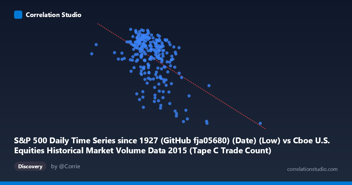
S&P 500 Daily Time Series since 1927 (GitHub fja05680) (Date) (Low) vs Cboe U.S. Equities Historical Market Volume Data 2015 (Tape C Trade Count)
- Pearson correlation (r)
- -0.5012
- Spearman correlation
- -0.3984
- p-value
- 0
- Sample size (n)
- 252
- 95% confidence interval
- -0.5884 to -0.4026
- Granger causality
- None
- Granger optimal lag
- 1
AI analysis
Analysis: S&P 500 Daily Low vs. Cboe Tape C Trade Count (2015)
1. Overall Relationship The scatterplot reveals a moderate negative relationship between the S&P 500 daily low price and the Cboe Tape C trade count across 2015. As the S&P 500 daily low increases, the number of Tape C trades tends to decrease. The linear regression equation (y = −0.000221x + 2216.57) confirms this inverse slope, suggesting that on days when the index trades at higher price levels, Tape C transaction volume (by count) is somewhat lower, and vice versa. Visually, the data forms a downward-sloping cloud, though with considerable scatter around the trend line.
2. Correlation Strength, Direction, and Causality The Pearson correlation of r = −0.50 indicates a moderate negative association. However, the R² of 0.2512 is the more sobering figure — only about 25% of the variance in Tape C trade counts is explained by the S&P 500 daily low, leaving 75% attributable to other factors entirely. The 95% confidence interval of [−0.59, −0.40] is meaningfully away from zero, and the p-value of effectively 0 (with N = 3,302) confirms this is not a chance finding. That said, statistical significance with large N can be misleading about practical importance. Critically, the Granger causality results show no significant predictive directionality in either direction (X→Y: F = 0.015, p = 0.903; Y→X: F = 0.085, p = 0.770), meaning that knowing yesterday's S&P low does not help predict today's trade count, and vice versa. The correlation is contemporaneous and associative, not temporally predictive.
3. Notable Patterns, Clusters, and Outliers The bulk of the data clusters between S&P 500 lows of roughly 600,000–900,000 and trade counts between 2,000–2,126, forming a relatively dense core. However, several notable features stand out. A handful of points at very high X-values (approaching 1,200,000–1,600,000) tend to have noticeably lower trade counts (around 1,867–1,971), pulling the regression line and driving much of the negative correlation — these appear to represent late-year sessions when the index traded at elevated levels. Conversely, the leftmost outlier near X = 291,078 (trade count ~2,059) is anomalous, likely representing an early-year or volatility-driven session. The upper-left region shows several high-trade-count days (2,100) occurring at relatively moderate price levels, hinting at elevated activity during periods of market stress or high volatility.
4. Confounding Factors and Caveats Several confounding factors complicate a straightforward interpretation. First, 2015 was a year with a notable late-summer volatility spike (August 2015 correction), which would simultaneously depress price levels and spike trade counts — this single episode could account for a disproportionate share of the observed correlation. Second, secular trends within the year mean both variables may be co-moving with time itself (e.g., rising prices through mid-year, falling prices in Q3), creating spurious correlation driven by a common temporal factor rather than a direct economic link. Third, Tape C specifically covers NYSE Arca-listed securities (predominantly ETFs), so the relationship may reflect ETF arbitrage activity during volatile periods rather than a broad market phenomenon. Finally, index price level is not the same as return or volatility, so interpreting this as a volatility-volume relationship would require a different variable specification.
5. Actionable Insights and Further Investigation Given the lack of Granger causality, practitioners should not attempt to use S&P 500 price levels as a leading indicator for Tape C trade flow, or vice versa. More productive next steps would include: (a) replacing the price level variable with intraday volatility (e.g., high-low range or VIX) to test whether uncertainty rather than price level drives trade count; (b) decomposing the time series to remove the shared temporal trend and re-testing the correlation on residuals to assess whether the relationship holds independently of the calendar drift; (c) isolating the August 2015 correction period as a subsample to quantify how much of the overall correlation it drives; and (d) expanding to multiple years to test whether this negative relationship is a stable structural feature or an artifact of 2015's specific price trajectory.
X dataset: Cboe U.S. Equities Historical Market Volume Data 2015
Y dataset: S&P 500 Daily Time Series since 1927 (GitHub fja05680) (Date)
Part of experiment: Daily - Cboe U.S. Equities Historical Market Volume Data 2015 vs S&P 500 Daily Time Series since 1927 (GitHub fja05680) (Date)