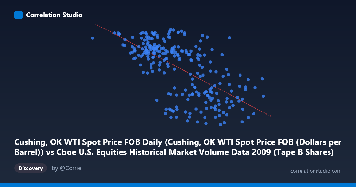
Cushing, OK WTI Spot Price FOB Daily (Cushing, OK WTI Spot Price FOB (Dollars per Barrel)) vs Cboe U.S. Equities Historical Market Volume Data 2009 (Tape B Shares)
- Pearson correlation (r)
- -0.6387
- Spearman correlation
- -0.6337
- p-value
- 0
- Sample size (n)
- 252
- 95% confidence interval
- -0.7065 to -0.5593
- Granger causality
- None
- Granger optimal lag
- 1
AI analysis
Analysis: WTI Crude Oil Prices vs. Cboe Tape B Share Volume (2009)
Relationship Overview The scatterplot reveals a moderately strong negative relationship between WTI crude oil spot prices (X-axis) and Cboe Tape B share volumes (Y-axis) across 252 trading days in 2009. As oil prices increase, Tape B equity share volumes tend to decline, and vice versa. The linear regression equation (y = -1.999×10⁻⁷x + 91.30) confirms this inverse slope, with the intercept anchoring predicted Tape B volumes around 91 shares (in relevant units) at zero oil price — a theoretical baseline. The overall scatter is substantial, suggesting the relationship, while real, is far from deterministic.
Correlation Strength and Statistical Reliability The Pearson correlation of r = -0.6387 indicates a moderate-to-strong negative association. The r² of 0.4079 means that roughly 40.8% of the variance in Tape B share volumes is statistically explained by WTI oil price levels — meaningful, but leaving nearly 60% of variation attributable to other factors. The 95% confidence interval of [-0.7065, -0.5593] is relatively tight and does not cross zero, reinforcing that this is a robust, non-trivial relationship. With a p-value effectively at zero and a sample of n = 252 drawn from a population of N = 3,232, the result is highly statistically significant. However, the Granger causality tests reveal no significant temporal predictive direction in either direction (X→Y: F = 0.002, p = 0.964; Y→X: F = 1.187, p = 0.277), meaning that while the two variables move together contemporaneously, neither reliably leads the other in time. This is a critical distinction: correlation here reflects co-movement, not forecastability.
Notable Patterns and Outliers Several features stand out in the data. There is a broad central cluster of observations where oil prices range roughly from ~$100M to ~$175M (in the X units provided) and Tape B volumes cluster between 60–80, suggesting a relatively stable regime for much of mid-2009. At higher oil price values (above ~$190M), volumes consistently compress toward the 37–55 range, forming a distinct lower-right cluster that drives much of the negative correlation. A few notable outliers are visible: the point near (33,822,027, 76.83) sits at an extremely low oil price with moderate-high volume, likely representing the early January 2009 period when oil had collapsed from 2008 highs. Similarly, points near (254,504,132, 56.67) and (243,585,656, 39.35) at the far right represent the late-year oil price recovery. The relationship also appears slightly non-linear — volumes seem to decline steeply once oil prices cross a threshold (~$160–170M range), potentially suggesting a regime-change effect rather than a purely linear dynamic.
Confounding Factors and Caveats Interpreting this correlation requires considerable caution. 2009 was an extraordinary macroeconomic year, dominated by the aftermath of the 2008 financial crisis, the U.S. economic stimulus package, and a dramatic V-shaped recovery in risk assets — all of which simultaneously affected both equity trading volumes and oil prices through common macro drivers (risk sentiment, economic recovery expectations, institutional reallocation). This creates a classic spurious correlation via shared confounding: both variables may simply be responding to the same underlying macro cycle rather than influencing one another. Additionally, Tape B specifically covers NYSE American (AMEX)-listed securities, a narrower market segment that may have idiosyncratic volume dynamics not representative of broader equity markets. The absence of Granger causality further supports the interpretation that the observed correlation is a coincident relationship driven by common external forces, not a structural link.
Actionable Insights and Further Investigation Despite the lack of Granger causality, the 40.8% explained variance is substantial enough to warrant deeper investigation. Recommended next steps include: (1) Controlling for macro variables — particularly VIX (fear index), S&P 500 returns, and Fed policy events — to determine how much of the correlation survives after accounting for shared crisis-recovery dynamics; (2) Extending the analysis beyond 2009 to test whether this relationship persists across different market regimes (e.g., 2010–2014 bull market, 2020 COVID shock), since a single-year correlation may be epoch-specific; (3) Applying a rolling correlation analysis to detect whether the relationship strengthens or reverses at different points in the year; (4) Testing non-linear models (e.g., piecewise regression or LOESS) given the apparent threshold behavior around mid-range oil prices; and (5) Investigating whether energy-sector stocks (which would appear in Tape B) disproportionately drive the volume signal, which would provide a more mechanistic explanation for the co-movement.
X dataset: Cboe U.S. Equities Historical Market Volume Data 2009
Y dataset: Cushing, OK WTI Spot Price FOB Daily
Part of experiment: Daily - Cboe U.S. Equities Historical Market Volume Data 2009 vs Cushing, OK WTI Spot Price FOB Daily