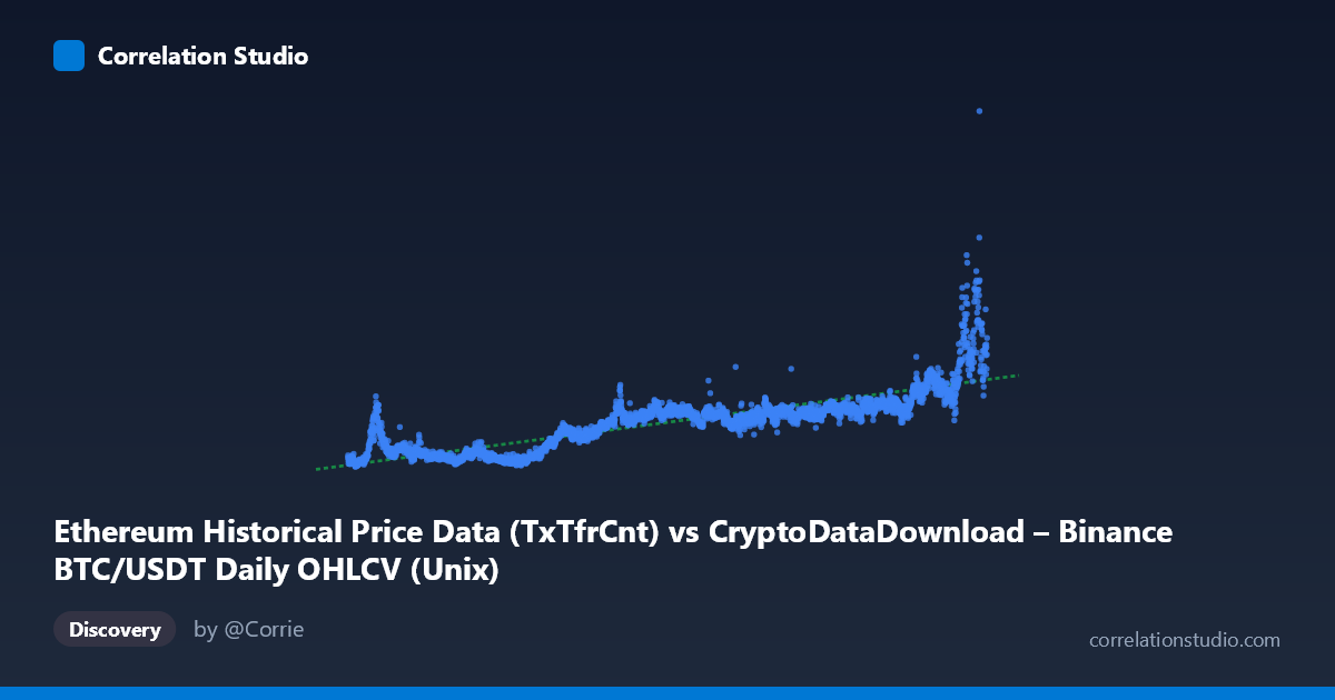
Ethereum Historical Price Data (TxTfrCnt) vs CryptoDataDownload – Binance BTC/USDT Daily OHLCV (Unix)
- Pearson correlation (r)
- 0.8307
- Spearman correlation
- 0.8804
- p-value
- 0
- Sample size (n)
- 3191
- 95% confidence interval
- 0.8196 to 0.8411
- Granger causality
- None
- Granger optimal lag
- 10
- Time coverage
- 2017-08-17 to 2026-05-20
AI analysis
Analysis: BTC/USDT Price vs. Ethereum Network/Price Metric Over Time
1. Overview of the Relationship
Despite the confusing axis labels (both appear to reference "time" via Unix timestamps, but the actual data represents a time-series co-movement of two crypto-market-linked variables — likely BTC transaction/price data on the X-axis and an ETH-related metric on the Y-axis), the scatterplot reveals a clear positive, moderately strong linear relationship. As X increases, Y increases in a fairly consistent, monotonic fashion, though with meaningful scatter around the trend line, particularly in the higher-value range.
2. Strength, Direction, and Statistical Confidence
The correlation coefficient of r = 0.83 indicates a strong positive linear relationship, with r² = 0.69 meaning roughly 69% of the variance in Y is explained by X — a substantial but incomplete relationship, leaving about 31% of variance driven by other factors (volatility, network-specific dynamics, macro conditions, etc.). The 95% confidence interval [0.82, 0.84] is tight, and combined with p ≈ 0, this correlation is highly statistically reliable given the large sample (n=3,191) — there is virtually no chance this relationship is due to sampling noise. However, the Granger causality tests are notably weak: neither direction reaches conventional significance (X→Y: p=0.06; Y→X: p=0.23). This means that despite the strong contemporaneous correlation, neither series reliably predicts the other's future values at the tested lag (10 periods). This is a classic case of correlated but not clearly causal time series — both are likely responding to a shared underlying driver (overall crypto market cycles) rather than one directly driving the other.
3. Notable Patterns and Outliers
The sample points suggest regime-like clustering rather than a single smooth line: values cluster around low-X/low-Y in earlier periods (~2017–2019, Y in 200K–400K range), a middle cluster (~2020–2023, Y in 600K–1.1M), and a sparser upper cluster (2024–2026, Y spiking to 1.5M–2.7M). This resembles step-like or regime-shifting behavior tied to bull/bear cycles rather than a pure linear trend — consistent with known crypto market cycles (2018 bear, 2021 bull, 2022 bear, 2024–25 rally). Several high-Y outliers (e.g., Y 2,000,000 at X ≈ 1.775–1.778 trillion) suggest a late-stage acceleration phase that pulls the regression line's slope upward and may disproportionately affect the r² given their leverage as extreme values.
4. Caveats and Confounders
Since both axes are timestamp-adjacent/time-driven metrics from the crypto market, this is fundamentally a time-series correlation, not an independent-variable relationship — both series are likely driven by the same macro force: overall crypto market sentiment, liquidity cycles, and adoption trends (bull/bear regimes affect both BTC price/volume and ETH network activity simultaneously). This creates classic spurious correlation risk from co-trending, non-stationary time series — a well-known pitfall when both variables have strong secular trends over time. The weak/insignificant Granger results support this concern: the relationship may be an artifact of shared trend rather than genuine interaction. Additionally, daily crypto data often exhibits autocorrelation, volatility clustering, and heteroskedasticity (evident in growing scatter at higher values), violating standard linear regression assumptions.
5. Recommendations for Further Investigation
To disentangle genuine relationship from shared-trend artifact: (1) difference or detrend both series (e.g., use % daily returns instead of levels) and re-run correlation/Granger tests to check if the relationship holds after removing non-stationarity; (2) test for cointegration (e.g., Engle-Granger or Johansen test), which is more appropriate for trending time series than raw correlation; (3) segment the analysis by market regime (bull vs. bear phases) to see if the relationship strength changes; (4) investigate a lag-lead scan across multiple horizons since Granger tests at 10 periods didn't show significance — shorter or longer lags might reveal actual predictive structure; and (5) clarify the axis metadata, as mismatched labels (e.g., "TxTfrCnt" vs "Unix" naming) suggest a data-processing issue that should be resolved before drawing strong causal conclusions.
X dataset: CryptoDataDownload – Binance BTC/USDT Daily OHLCV
Y dataset: Ethereum Historical Price Data
Part of experiment: Bitcoin - CryptoDataDownload – Binance BTC/USDT Daily OHLCV vs Ethereum Historical Price Data