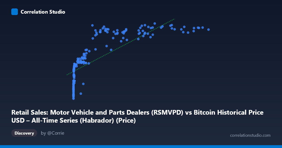
Retail Sales: Motor Vehicle and Parts Dealers (RSMVPD) vs Bitcoin Historical Price USD – All-Time Series (Habrador) (Price)
- Pearson correlation (r)
- 0.8168
- Spearman correlation
- 0.9588
- p-value
- 0
- Sample size (n)
- 189
- 95% confidence interval
- 0.7631 to 0.8594
- Granger causality
- None
- Granger optimal lag
- 10
AI analysis
Analysis: Bitcoin Price vs. Motor Vehicle & Parts Retail Sales
1. What the Visualization Reveals
The scatterplot shows a strong positive association between Bitcoin's historical price and U.S. retail sales for motor vehicle and parts dealers. However, the relationship is clearly non-linear: at low Bitcoin prices (under ~$1,000), retail sales cluster tightly between $61,000–$100,000, while as Bitcoin price climbs into the tens of thousands, retail sales rise but with diminishing marginal increases — the curve flattens at the high end (retail sales plateau around $130,000–$142,000 even as Bitcoin ranges from $30,000 to $118,000). This log-like saturation pattern is typical when one variable grows exponentially (Bitcoin price) while the other grows linearly/steadily (retail sales driven by inflation, population, and economic growth).
2. Strength, Direction, and Uncertainty
The Pearson correlation (r = 0.817, r² = 0.667) indicates a strong positive linear relationship, with roughly 67% of the variance in retail sales "explained" by Bitcoin price in a linear model. The 95% CI [0.763, 0.859] is fairly tight and excludes zero, and the p-value ≈ 0 confirms this is not a chance finding within the sample. However, the note that Spearman's ρ exceeds Pearson's r confirms the visual impression: a log or power-law transformation of Bitcoin price would likely fit better than the linear model, and the true explanatory power of the shape of the relationship is probably higher than r² suggests.
Critically, the Granger causality tests show no significant predictive direction in either direction (X→Y: p = 0.89; Y→X: p = 0.56). This means neither variable's past values help forecast the other's future values in a time-series sense, despite the strong contemporaneous correlation. This is a crucial distinction: correlation here reflects shared trends over time, not one variable driving or predicting the other.
3. Notable Patterns and Outliers
The data shows two distinct regimes: a dense low-X cluster (Bitcoin < $2,000, spanning 2010–2017) where retail sales vary substantially (65,000–100,000) with weak Bitcoin sensitivity, and a sparser high-X cluster (Bitcoin $20,000, 2020 onward) where retail sales sit consistently high (117,000–142,000). There's little data in the "middle" (Bitcoin $2,000–$20,000), creating a somewhat bimodal distribution that can inflate the apparent linear correlation. No extreme outliers are evident, but the point (56,973, 118,762) sits noticeably below the trend of nearby high-Bitcoin points, suggesting some sales volatility (possibly a COVID-related dip) independent of price.
4. Confounding Factors and Caveats
This is a textbook case of spurious correlation via shared temporal trends. Both series have risen substantially since 2010–2026: Bitcoin due to speculative adoption cycles, and retail auto sales due to inflation, nominal price growth, and general economic expansion — not because one causes the other. Both are non-stationary time series (trending upward over 15+ years), which is well-known to inflate Pearson correlation even between economically unrelated variables. The Granger non-causality result reinforces that this is likely a coincidental co-trending relationship rather than a causal or even predictive one.
5. Suggestions for Further Investigation
Analysts should detrend or difference both series (e.g., use month-over-month % changes rather than levels) and recompute correlation — this is the standard remedy for spurious trend-driven correlation in time series. Fitting a log-linear or power model (log(X) vs Y) would better capture the apparent saturation curve and likely improve fit. Given the lack of Granger causality, this pairing is not suitable for building a predictive trading or economic model; instead, treat both as independently trending series likely driven by macroeconomic conditions (e.g., overall consumer spending growth, USD inflation, or interest rate cycles) and consider testing each against a common macro driver (GDP, CPI, M2 money supply) to identify genuine causal structure.
X dataset: Bitcoin Historical Price USD – All-Time Series (Habrador)
Y dataset: Retail Sales: Motor Vehicle and Parts Dealers
Part of experiment: Bitcoin - Bitcoin Historical Price USD – All-Time Series (Habrador) vs Retail Sales: Motor Vehicle and Parts Dealers