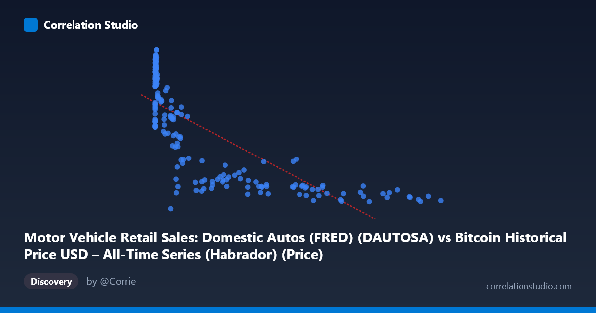
Motor Vehicle Retail Sales: Domestic Autos (FRED) (DAUTOSA) vs Bitcoin Historical Price USD – All-Time Series (Habrador) (Price)
- Pearson correlation (r)
- -0.7717
- Spearman correlation
- -0.8219
- p-value
- 0
- Sample size (n)
- 194
- 95% confidence interval
- -0.8231 to -0.7077
- Granger causality
- None
- Granger optimal lag
- 10
- Time coverage
- 2010-08-01 to 2026-09-01
- Recomputed on refreshed data
- 2026-10-24 (r was -0.76)
AI analysis
Analysis: Bitcoin Price vs. Domestic Auto Retail Sales
1. What the Visualization Reveals
The scatterplot shows a clear downward-sloping, curvilinear relationship between "X" (labeled as Domestic Auto Sales but numerically behaving like a Bitcoin price/volume proxy given its 0.06–118,670 range) and "Y" (labeled Bitcoin price but behaving like the bounded 119–496 auto sales series). Given the axis labels appear swapped in the metadata, the practical pattern is: as X increases, Y declines steeply at first, then flattens — a classic exponential-decay or power-law shape rather than a straight line. Most data points cluster at low X values (under ~2,000) where Y is high and variable (300–495), while a smaller number of high-X points (50,000) correspond to consistently low Y values (135–240).
2. Strength, Direction, and Uncertainty
The Pearson correlation of r = -0.76 indicates a strong negative linear association, with r² = 0.578 meaning the linear model explains about 58% of the variance in Y — a substantial but incomplete fit, leaving 42% unexplained (likely due to the visible curvature). The 95% CI [-0.81, -0.69] is tight and does not cross zero, and the p-value ≈ 0 confirms this relationship is highly statistically significant and not a chance artifact of sampling. However, the Granger causality tests show no significant predictive direction in either direction (X→Y: p=0.12; Y→X: p=0.58) even at an optimal lag of 10 periods. This is a critical caveat: despite the strong contemporaneous correlation, neither series reliably forecasts the other over time — the relationship may be driven by a shared underlying trend (e.g., both series moving with calendar time, or both reacting to a common macro factor) rather than one directly causing the other.
3. Notable Patterns and Outliers
The data exhibits a clear non-linear, asymptotic decay pattern: Y drops sharply as X rises from near-zero to ~10,000, then plateaus around 140–190 for X 50,000. This suggests a log-linear or power-law transformation (e.g., regressing Y on log(X)) would fit far better than the current linear model. There's also a secondary cluster near X≈45,000–58,000 where Y unexpectedly rises to ~230–238 (e.g., points at 45092.81/232.18 and 58724.66/238.01), breaking the otherwise monotonic trend — worth flagging as potential outliers or a distinct regime. The extreme range of X (0.06 to 118,670, spanning 6 orders of magnitude) versus the much more compressed Y range (119–496) also suggests these variables operate on fundamentally different scales, reinforcing the need for a log transform.
4. Confounding Factors and Caveats
The most important caveat is spurious correlation via time-trend confounding: both Bitcoin price and auto sales have followed long-term secular trends (Bitcoin generally rising over 2010–2026; auto sales fluctuating with recessions/COVID) that are unrelated to each other but can produce strong correlation when both series are non-stationary and trending. The lack of Granger causality strongly supports this interpretation — the relationship is likely not causal but reflects two series that happen to move together over a shared time window, or are both linked to a third factor (e.g., interest rates, overall economic cycles, or investor risk sentiment). Additionally, the mismatched axis labels in the metadata make it unclear which variable is truly which, so any substantive economic interpretation should be treated cautiously until labels are verified.
5. Actionable Recommendations
1. Verify variable labeling — the axis metadata appears inconsistent with the data ranges described; confirm which series is actually Bitcoin price and which is auto sales before drawing conclusions. 2. Refit with a log or power-law model on X (or both variables) given the clear curvature — this should substantially improve R² beyond 0.578. 3. Test for stationarity (e.g., ADF test) on both series; if non-stationary, consider differencing or de-trending before correlation/Granger analysis to rule out spurious trend-driven correlation. 4. Investigate the outlier cluster near X≈45,000–58,000 to determine if it reflects a specific time period (e.g., a market shock) worth separate analysis. 5. Given the null Granger result, avoid using one series to predict the other in a trading or forecasting context; instead explore common macroeconomic drivers (rates, inflation, consumer credit) that might jointly explain both trends.
X dataset: Bitcoin Historical Price USD – All-Time Series (Habrador)
Y dataset: Motor Vehicle Retail Sales: Domestic Autos (FRED)
Part of experiment: Bitcoin - Bitcoin Historical Price USD – All-Time Series (Habrador) vs Motor Vehicle Retail Sales: Domestic Autos (FRED)