World Bank CO2 Emissions by Country (DataBank) (Solid Fuel) vs US Employment and Unemployment (population)
- Pearson correlation (r)
- 0.9186
- Spearman correlation
- 0.8733
- p-value
- 0
- Sample size (n)
- 80
- 95% confidence interval
- 0.8756 to 0.9471
- Granger causality
- None
- Granger optimal lag
- 10
AI analysis
Scatterplot Analysis: Solid Fuel CO2 Emissions vs. US Population
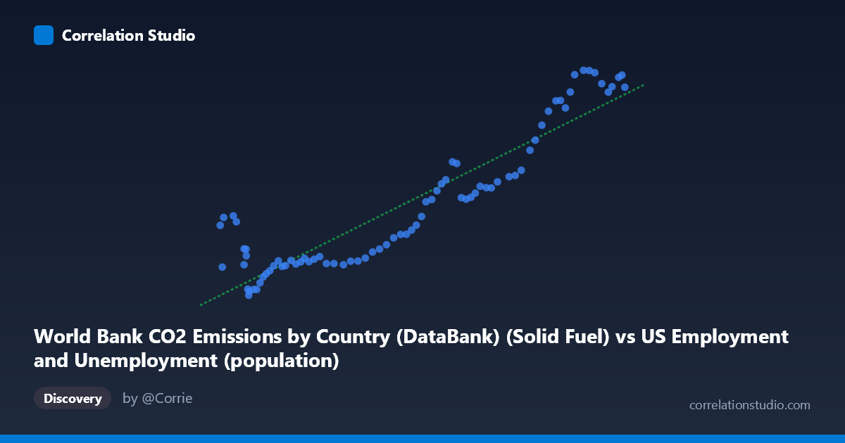
1. Overall Relationship The scatterplot reveals a strong, positive relationship between solid fuel CO2 emissions (X-axis, drawn from US Employment/Unemployment data) and US population figures (Y-axis, drawn from World Bank CO2 data). As solid fuel emissions increase across the observed range of approximately 93,220 to 260,329 units, population values rise correspondingly from roughly 9,555 to 31,154 units. The linear regression equation (y = 0.115435x − 1,206.86) describes a modest slope, meaning each unit increase in solid fuel emissions corresponds to roughly 0.115 units of population increase — though the practical interpretation of this magnitude depends heavily on the underlying units of measurement for both variables.
2. Correlation Strength, Direction, and Causality The Pearson correlation of r = 0.9186 indicates a very strong positive association, and the R² of 0.8438 means that approximately 84.4% of the variance in the population measure is statistically explained by variation in solid fuel emissions. This is a remarkably high explanatory share for a bivariate model. The 95% confidence interval for r [0.8756, 0.9471] is narrow and sits entirely in strongly positive territory, and the p-value ≈ 0 (with n = 80 paired observations) confirms this correlation is highly statistically significant — the probability of observing this result by chance under a null hypothesis of no relationship is essentially zero. However, Granger causality tests in both directions fail to reach significance (X→Y: F = 1.005, p = 0.453; Y→X: F = 1.197, p = 0.316), with an optimal lag of 10 periods. This means that, despite the strong contemporaneous correlation, neither variable temporally predicts the other beyond what each predicts from its own past values. The correlation is strong, but it carries no detectable directional forecasting power.
3. Notable Patterns, Clusters, and Outliers The data from 1941–2020 naturally segments into several visible clusters. Lower X values (roughly 93,000–140,000) show tightly grouped, relatively low Y values with modest scatter, likely corresponding to mid-20th century decades when both industrial emissions and population were smaller. The middle range (140,000–210,000) shows a broader spread, suggesting a transitional period where the relationship becomes noisier. The upper cluster (230,000–260,000) shows high Y values with relatively tight grouping again, consistent with late 20th/early 21st century conditions. A few points in the lower-X range show elevated Y values (e.g., points near X ≈ 93,220–99,900 with Y ≈ 16,000–17,000), which sit noticeably above the regression line — these may represent years where population was relatively high despite lower recorded solid fuel emissions, hinting at potential structural breaks or data anomalies. Similarly, some mid-range X values yield lower-than-predicted Y values, suggesting the linear fit, while strong overall, is not uniformly accurate across the full range.
4. Confounding Factors and Caveats The most significant caveat here is the dataset label mismatch: the X-axis is labeled as a solid fuel CO2 emissions column sourced from a US employment dataset, while the Y-axis is a population column sourced from a CO2 emissions dataset. This cross-dataset column attribution is highly irregular and strongly suggests these variables are both functioning as proxies for time — both solid fuel emissions and US population grew monotonically or near-monotonically across most of the 1941–2020 period, meaning their correlation largely reflects shared temporal trend (spurious correlation) rather than any direct causal or mechanistic link. The failure of Granger causality in both directions supports this interpretation. Additionally, with annual time-series data over 80 years, autocorrelation within each series is virtually guaranteed, which inflates effective sample size assumptions and makes traditional significance thresholds overly optimistic. Structural changes — WWII industrial ramp-up, post-war economic booms, the energy transitions of the 1970s, and 21st-century emission plateaus — could all introduce non-stationarity that distorts a single linear model.
5. Actionable Insights and Further Investigation Given the likely spurious nature of this correlation, the most important next step is detrending both series (e.g., via first-differencing or HP filtering) before drawing any substantive conclusions; a correlation of year-over-year changes would be far more informative than the level correlation. Researchers should also verify the dataset column assignments, as the cross-sourced labeling raises data pipeline concerns that could invalidate the analysis entirely. If the relationship is genuine, per-capita emissions analysis would be more meaningful than raw totals, effectively removing the population scaling effect. Extending the Granger causality analysis with shorter lag windows or cointegration tests (e.g., Engle-Granger or Johansen) would better characterize the long-run relationship between two potentially non-stationary series. Finally, incorporating energy-mix transition variables (renewables share, natural gas substitution) as controls could help isolate whether any portion of this relationship survives beyond the common time trend.
X dataset: US Employment and Unemployment
Y dataset: World Bank CO2 Emissions by Country (DataBank)
Part of experiment: Yearly - US Employment and Unemployment vs World Bank CO2 Emissions by Country (DataBank)