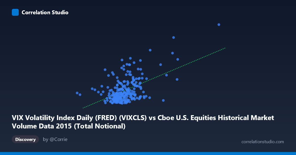
VIX Volatility Index Daily (FRED) (VIXCLS) vs Cboe U.S. Equities Historical Market Volume Data 2015 (Total Notional)
- Pearson correlation (r)
- 0.5151
- Spearman correlation
- 0.368
- p-value
- 0
- Sample size (n)
- 252
- 95% confidence interval
- 0.4182 to 0.6005
- Granger causality
- None
- Granger optimal lag
- 1
AI analysis
Analysis: VIX Volatility Index vs. Total Notional Market Volume (2015)
Relationship Overview The scatterplot reveals a positive relationship between the CBOE VIX Volatility Index and total notional market volume in U.S. equities for 2015. The linear regression equation (y = 5.25×10⁻¹⁰x + 5.52) confirms that as market volume (notional value) increases, implied volatility tends to rise as well. This aligns strongly with financial theory: periods of heightened uncertainty and fear drive both increased trading activity and elevated implied volatility, as market participants hedge positions and react to rapidly shifting information. The relationship is most visibly concentrated in the lower-left region of the plot, with a meaningful upward sweep as volume grows large.
Correlation Strength and Statistical Significance The Pearson correlation of r = 0.5151 indicates a moderate positive association, but the explanatory power is more modest than the raw correlation suggests: r² = 0.2653 means only ~26.5% of variance in VIX is explained by notional volume, leaving roughly three-quarters of VIX variation attributable to other factors. The 95% confidence interval of [0.418, 0.601] is reasonably tight and entirely positive, and with a p-value effectively at zero (population N = 3,302, sample n = 252), this correlation is unambiguously statistically significant — not a sampling artifact. However, statistical significance here should not be conflated with strong predictive power. Critically, the Granger causality tests reveal no significant temporal predictive direction in either direction (X→Y: F = 0.128, p = 0.72; Y→X: F = 0.017, p = 0.90), meaning that knowing today's volume does not meaningfully help predict tomorrow's VIX, and vice versa. The two variables move together but neither reliably leads the other at a one-period lag.
Patterns, Clusters, and Outliers Several structural features stand out in the data. The bulk of observations cluster tightly in the x-range of approximately 15–25 billion (notional volume) with VIX values between 12 and 22, forming a dense core consistent with normal 2015 market conditions. However, there is a visible upper-right tail of high-leverage points — notably observations near (35.6B, 36.0), (36.8B, 28.0), and (48.9B, ~40) — which correspond almost certainly to the late-August 2015 market volatility spike when Chinese devaluation fears triggered a sharp global selloff. These extreme outliers exert disproportionate influence on the regression line and correlation coefficient. There is also a notable lower-right anomaly around (25.7B, 14.0), where high volume coincided with surprisingly low VIX, suggesting a high-volume day without fear — possibly a post-volatility reversion or index rebalancing event.
Confounding Factors and Caveats Several important caveats apply. First, the August 2015 volatility cluster likely inflates the correlation substantially — if those outlier sessions were removed, r would likely drop meaningfully, making this a leverage-driven relationship rather than a stable structural one. Second, directionality is ambiguous: it is equally plausible that high VIX causes high volume (fear drives trading) as the reverse, and the Granger test confirms neither direction dominates temporally. Third, notional volume conflates price and quantity — on high-VIX days, prices themselves are elevated or erratic, mechanically inflating notional values even if share count traded is unchanged. This introduces an endogenous measurement artifact. Finally, the 2015 sample covers only a single calendar year, limiting generalizability, and the relationship may behave very differently in bear markets, low-volatility regimes, or post-COVID structural market changes.
Actionable Insights and Further Investigation Despite the caveats, this analysis yields practical directions. Researchers should re-run the correlation excluding the August 2015 spike to isolate the "normal regime" relationship from the tail-driven signal. Investigating volume decomposed by share count vs. notional value would clarify whether the correlation is structural or price-mechanical. Given the failed Granger causality, same-day (contemporaneous) regime models — such as hidden Markov models distinguishing low- and high-volatility states — would likely outperform simple lag-based predictions. Extending the dataset across multiple years (particularly including 2018 and 2020 volatility events) would test whether the r ≈ 0.52 relationship is stable or episodic. Finally, incorporating options volume, put/call ratios, or bid-ask spreads as covariates could help disentangle fear-driven volume from liquidity-driven volume, potentially explaining much of the remaining 73.5% variance.
X dataset: Cboe U.S. Equities Historical Market Volume Data 2015
Y dataset: VIX Volatility Index Daily (FRED)
Part of experiment: Daily - Cboe U.S. Equities Historical Market Volume Data 2015 vs VIX Volatility Index Daily (FRED)