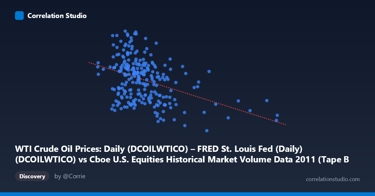
WTI Crude Oil Prices: Daily (DCOILWTICO) – FRED St. Louis Fed (Daily) (DCOILWTICO) vs Cboe U.S. Equities Historical Market Volume Data 2011 (Tape B Notional)
- Pearson correlation (r)
- -0.4013
- Spearman correlation
- -0.3527
- p-value
- 0
- Sample size (n)
- 252
- 95% confidence interval
- -0.5001 to -0.2923
- Granger causality
- None
- Granger optimal lag
- 1
AI analysis
Analysis: WTI Crude Oil Prices vs. Cboe Tape B Notional Trading Volume (2011)
Relationship Overview The scatterplot reveals a moderate negative relationship between WTI crude oil prices (x-axis) and Cboe Tape B notional trading volume (y-axis) across 252 trading days in 2011. The linear regression equation (y = -1.806×10⁻⁹x + 104.11) confirms that as oil prices rise, Tape B notional volume tends to decline. Visually, the cloud of points slopes gently downward from left to right, though considerable scatter is present throughout, suggesting the relationship is real but far from deterministic. The bulk of observations cluster in the 3–7 billion range on the x-axis and 85–110 on the y-axis, with a discernible thinning of the upper-right quadrant.
Correlation Strength and Statistical Significance The Pearson correlation of r = -0.40 indicates a moderate negative association, but the explanatory power is modest: R² = 0.161, meaning only about 16% of the variance in Tape B notional volume is attributable to variation in oil prices, leaving 84% unexplained by this relationship alone. The 95% confidence interval for r of [-0.50, -0.29] is entirely negative and does not cross zero, reinforcing directional confidence. The p-value of 3.59×10⁻¹¹ is highly significant at N = 3,780, confirming this is extremely unlikely to be a chance finding. However, Granger causality analysis finds no significant predictive directionality in either direction — neither X→Y (F = 0.057, p = 0.811) nor Y→X (F = 2.303, p = 0.130) reaches significance at conventional thresholds. This is a critical nuance: while a contemporaneous statistical association exists, neither variable demonstrably leads the other temporally, undermining any mechanistic or forecasting interpretation.
Notable Patterns, Clusters, and Outliers Several features stand out in the sample points. There are notable high-volume outliers at lower oil price ranges — for instance, points near x ≈ 3.06B with y = 111.68 and x ≈ 5.27B with y = 110.60, suggesting periodic spikes in Tape B volume independent of oil price levels. Conversely, low-volume observations appear at both moderate and high oil prices (e.g., x ≈ 6.10B, y = 78.93; x ≈ 6.06B, y = 81.87), hinting at possible regime changes or specific event-driven suppression of equity trading. The far-right tail (x 8B, representing elevated oil price periods) shows relatively compressed y-values clustering around 85–98, consistent with the negative trend but also suggesting reduced trading activity during high-oil-price stress periods in 2011, plausibly tied to the Arab Spring and associated commodity shocks.
Confounding Factors and Caveats Interpreting this correlation requires significant caution. 2011 was an unusually volatile year — the European sovereign debt crisis, U.S. debt ceiling standoff, Arab Spring, and the Fukushima disaster all created distinct market regimes that could independently affect both oil prices and equity trading volumes. The absence of Granger causality suggests the observed correlation may be a spurious co-movement driven by shared macro risk factors (e.g., risk-off sentiment simultaneously depressing trading activity and elevating oil as a safe-haven/commodity hedge) rather than any direct causal link. Additionally, Tape B specifically covers NYSE MKT (AMEX) and regional exchange stocks — a narrower market segment that may respond differently to macroeconomic signals than broader indices. Temporal autocorrelation in both daily oil prices and trading volumes could also inflate apparent significance.
Actionable Insights and Further Investigation Given the modest explanatory power and absent Granger causality, this correlation should not be used for predictive modeling in isolation. However, the finding warrants deeper investigation: (1) Segment the analysis by macro-event regimes (pre/post-August 2011 debt ceiling crisis) to test whether the correlation is driven by a specific sub-period; (2) Introduce control variables such as VIX (volatility index), S&P 500 returns, or USD index to test whether the oil-volume relationship survives multivariate adjustment; (3) Test non-linear specifications — the scatter hints at possible threshold effects at extreme oil price levels; (4) Replicate across other market tapes (Tape A, C) to determine whether the pattern is unique to Tape B or systemic; and (5) consider wavelet or rolling-window correlation analysis to detect whether the relationship strengthens during specific stress episodes, which would be actionable for risk monitoring frameworks.
X dataset: Cboe U.S. Equities Historical Market Volume Data 2011
Y dataset: WTI Crude Oil Prices: Daily (DCOILWTICO) – FRED St. Louis Fed (Daily)
Part of experiment: Daily - Cboe U.S. Equities Historical Market Volume Data 2011 vs WTI Crude Oil Prices: Daily (DCOILWTICO) – FRED St. Louis Fed (Daily)