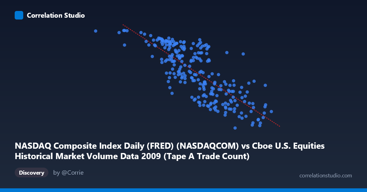
NASDAQ Composite Index Daily (FRED) (NASDAQCOM) vs Cboe U.S. Equities Historical Market Volume Data 2009 (Tape A Trade Count)
- Pearson correlation (r)
- -0.7866
- Spearman correlation
- -0.7952
- p-value
- 0
- Sample size (n)
- 252
- 95% confidence interval
- -0.8296 to -0.7345
- Granger causality
- None
- Granger optimal lag
- 10
AI analysis
Scatterplot Analysis: NASDAQ Composite Index vs. Cboe Tape A Trade Count (2009)
Relationship Overview
The scatterplot reveals a clear negative relationship between the NASDAQ Composite Index daily closing values (X-axis) and the Cboe U.S. Equities Tape A Trade Count (Y-axis) across the 2009 trading year. As the NASDAQ index rises from its early-2009 lows (with values as low as ~362,081 in index-scaled units) toward year-end recovery levels approaching 2,549,192, the corresponding Tape A trade counts decline from peaks near 2,291 down to lows around 1,268–1,358. The linear regression equation y = −0.000546x + 2,735.36 captures this inverse trajectory well, and the downward slope is visually consistent across the full data range. This pattern likely reflects the market dynamics of 2009: extreme panic-driven trading volumes during the market bottom in early 2009, followed by a sustained rally in which prices rose but trading frenzy subsided.
Correlation Strength and Statistical Significance
The correlation of r = −0.7866 is strong and highly statistically significant (p ≈ 0, N = 3,232, n = 252). The 95% confidence interval of [−0.8296, −0.7345] is relatively narrow, confirming the robustness of this estimate and ruling out the possibility of a weak or negligible relationship. The coefficient of determination R² = 0.6188 means that approximately 61.9% of the variance in Tape A trade counts is explained by the NASDAQ index level — a substantial but not total explanatory share, indicating meaningful additional factors are at play in the remaining ~38%. Despite this strong contemporaneous correlation, the Granger causality tests are non-significant in both directions (X→Y: F = 1.75, p = 0.072; Y→X: F = 1.56, p = 0.121). This is an important nuance: while the two variables move together, neither one demonstrably predicts the other at the tested lag of 10 periods in a temporal sense. The relationship is associative rather than directionally predictive at this timescale.
Notable Patterns, Clusters, and Outliers
Several structural features stand out in the data. At the lower end of the X-axis (index values below ~800,000), trade counts cluster at elevated levels (2,100–2,291), consistent with the market stress environment of early 2009. Two notable high-leverage points appear near X = 362,081 (Y ≈ 2,285) and X = 712,211 (Y ≈ 2,291) — these likely represent the market's capitulation period in late February/early March 2009, during the post-financial-crisis trough. At the upper end of the X range (~2,400,000–2,549,192), trade counts drop to their lowest observed values (~1,293–1,441), reflecting the calmer, recovering market conditions of late 2009. There is also modest but visible scatter around the regression line in the mid-range of NASDAQ values (roughly 1,500,000–2,000,000), suggesting the relationship is somewhat heteroscedastic — the spread of trade counts appears wider in the moderate index zone, perhaps reflecting transitional market conditions between fear-driven and confidence-driven trading regimes.
Confounding Factors and Interpretive Caveats
Several important caveats apply. First, this correlation is temporally confounded: both variables are time series evolving across 2009, so the negative correlation may largely reflect the shared time trend (market recovery) rather than a direct structural link between index level and trade count. A spurious or partially spurious correlation driven by common macroeconomic drivers — the post-crisis recovery, Federal Reserve interventions, and stabilizing credit markets — cannot be ruled out. Second, Tape A specifically covers NYSE-listed securities, while the NASDAQ index reflects NASDAQ-listed stocks; any cross-venue routing dynamics or exchange competition effects could distort the relationship. Third, the failed Granger causality tests suggest that even if the levels are correlated, the day-to-day movements do not show a leading/lagging directional relationship, which cautions against interpreting the correlation as mechanistically causal. Finally, data aggregation at the daily level may mask intraday volatility patterns or within-day volume surges that would alter interpretation.
Actionable Insights and Further Investigation
For practitioners, this analysis suggests that elevated trade counts on Tape A may serve as a rough contemporaneous signal of depressed index levels, consistent with the well-established "volume spikes at bottoms" phenomenon in market microstructure research. However, since Granger causality is absent, trade counts should not be used naively as a leading predictor of index direction at 10-day lags. Further investigation should include: (1) detrending both series to remove the shared 2009 recovery trend and re-testing correlation on residuals; (2) expanding to multiple years to determine whether this negative relationship holds outside crisis periods or is specific to bear-market recovery dynamics; (3) testing shorter lag windows (1–3 days) in Granger tests, as the 10-period optimal lag may be too long to capture reactive trading behavior; and (4) comparing Tape A, B, and C trade counts separately against NASDAQ to isolate any cross-listing effects. Including volatility measures (e.g., VIX) as a control variable would help determine whether volatility is the true common driver underlying both the index decline and the elevated trade activity.
X dataset: Cboe U.S. Equities Historical Market Volume Data 2009
Y dataset: NASDAQ Composite Index Daily (FRED)
Part of experiment: Daily - Cboe U.S. Equities Historical Market Volume Data 2009 vs NASDAQ Composite Index Daily (FRED)