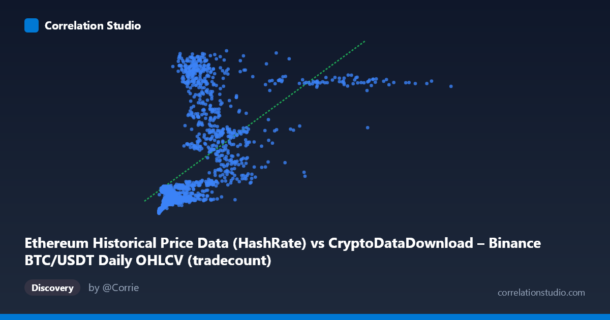
Ethereum Historical Price Data (HashRate) vs CryptoDataDownload – Binance BTC/USDT Daily OHLCV (tradecount)
- Pearson correlation (r)
- 0.5862
- Spearman correlation
- 0.7217
- p-value
- 0
- Sample size (n)
- 1855
- 95% confidence interval
- 0.5555 to 0.6153
- Granger causality
- X → Y
- Granger optimal lag
- 2
- Time coverage
- 2017-08-17 to 2022-09-14
AI analysis
Analysis: X (Ethereum "HashRate" proxy) vs. Y (BTC/USDT tradecount)
1. What the Visualization Reveals
The scatterplot shows a moderate positive association between the X variable (labeled as Ethereum hash rate data, though the mislabeling with BTC/USDT metadata suggests some data pipeline confusion worth flagging) and Y (tradecount). Points cluster heavily in the lower-left region (X < 1,000,000), where Y values mostly sit between 100-300, while a sparser scatter of higher-X points extends toward higher Y values. The relationship appears to fan out — variance in Y increases as X increases — rather than following a tight linear band.
2. Strength, Direction, and Statistical Confidence
The Pearson correlation (r = 0.586) indicates a moderate positive relationship, with r² = 0.344 meaning only about 34% of the variance in Y is explained by X — leaving roughly two-thirds of Y's variability unaccounted for by this single predictor. The 95% CI [0.556, 0.615] is fairly tight given the large sample (n=1,855), and the p-value of ~0 confirms the correlation is statistically robust and not due to chance. However, statistical significance here reflects sample size more than practical predictive strength — r² of 0.34 is a moderate, not strong, explanatory relationship.
The Granger causality results add a temporal dimension: X→Y is significant (F=3.56, p=0.029) while Y→X is not (p=0.084). This suggests past values of X have modest but statistically meaningful predictive power over future Y values, with lag-2 as optimal — but the effect is weak (F-statistic barely clears significance) and should not be overinterpreted as strong forecasting utility. It's directional evidence, not proof of strong causal mechanism.
3. Notable Patterns and Outliers
Several features stand out: - Heteroscedasticity: Spread in Y widens considerably as X increases — visible in points like (2,467,372 → 939.71) and (6,593,178 → 895.64) sitting far above the regression line's predicted values, while similar-X points elsewhere (e.g., 1,608,176 → 165.48) sit far below it. - Dense low-X cluster: The majority of points (X < 1M) show Y values compressed in a narrow 100-300 band, suggesting a floor/threshold effect at low X. - High-leverage outliers: A few extreme X values (4,545,385 and 8,860,928 max) sit far from the bulk of the data and could disproportionately influence both r and the regression slope. - Non-linear signal: The note that Spearman ρ exceeds Pearson r strongly suggests the true relationship is curved (likely logarithmic or power-law), consistent with the fan-shaped spread — common when both variables are wide-ranging financial/network metrics.
4. Confounding Factors and Caveats
- Data labeling inconsistency: The X-axis is labeled "Ethereum Historical Price Data (HashRate)" but sourced from a Binance BTC/USDT OHLCV dataset, while Y ("tradecount") is attributed to Ethereum data — this cross-labeling raises concerns about whether the actual variables being compared are correctly identified, which materially affects interpretation. - Time-series autocorrelation: Both crypto price/volume/hashrate metrics are highly autocorrelated over time (2017-2022 span includes multiple bull/bear cycles). Much of the "correlation" may reflect shared trends (e.g., both rising during 2020-2021 bull run) rather than a direct mechanical relationship — a classic spurious correlation risk with non-stationary time series. - Scale mismatch: X's huge range (2,153 to 8,860,928) with high stdev relative to mean indicates strong right-skew; a few large values can dominate linear correlation estimates. - N vs. n discrepancy: Population N=3,212 vs. paired sample n=1,855 implies ~42% of data was dropped (likely missing-value alignment), which could bias the sample if missingness isn't random across time.
5. Actionable Insights
1. Verify variable labels before drawing further conclusions — confirm whether X truly represents hash rate or price/volume, given the metadata conflict. 2. Log-transform both axes and refit — given the skewness and Spearman/Pearson divergence, a log-log or log-linear model will likely capture the relationship better than r²=0.34 suggests. 3. Test for stationarity (ADF/KPSS) and consider differencing the series before Granger causality testing, since raw price/volume trends in crypto are typically non-stationary and can produce misleading causality signals. 4. Segment by market regime (bull vs. bear periods) to check if the X→Y relationship holds consistently or is driven by specific 2020-2021 bull-market co-movement. 5. Investigate outliers (e.g., the 4.5M and 8.9M X-value points) individually — determine if they represent data errors, exchange anomalies, or genuine extreme network activity.
X dataset: CryptoDataDownload – Binance BTC/USDT Daily OHLCV
Y dataset: Ethereum Historical Price Data
Part of experiment: Bitcoin - CryptoDataDownload – Binance BTC/USDT Daily OHLCV vs Ethereum Historical Price Data