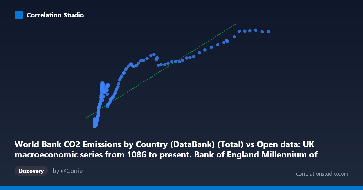
World Bank CO2 Emissions by Country (DataBank) (Total) vs Open data: UK macroeconomic series from 1086 to present. Bank of England Millennium of Macroeconomic Data. (Year) (value)
- Pearson correlation (r)
- 0.8554
- Spearman correlation
- 0.903
- p-value
- 0
- Sample size (n)
- 266
- 95% confidence interval
- 0.8194 to 0.8847
- Granger causality
- Y → X
- Granger optimal lag
- 10
AI analysis
Analysis of UK Macroeconomic Indicators vs. CO₂ Emissions (1751–2016)
1. What the Visualization Reveals
The scatterplot displays a moderately strong positive relationship between World Bank CO₂ emissions totals (X-axis) and UK Bank of England macroeconomic series values (Y-axis) across 266 paired observations spanning 1751 to 2016. The linear regression equation y = 0.0975x + 7107.94 suggests that for every unit increase in CO₂ emissions, the macroeconomic indicator rises by roughly 0.098 units, with a meaningful baseline intercept. The overall trajectory is clearly upward, consistent with the well-documented historical co-evolution of industrial output, energy consumption, and economic growth — particularly through the Industrial Revolution and twentieth-century expansion.
2. Correlation Strength, Direction, and Causality
The Pearson correlation of r = 0.8554 is strong and statistically unambiguous (p ≈ 0), with a tight 95% confidence interval of [0.819, 0.885] that leaves little room for chance. More practically, r² = 0.7317 means 73.2% of the variance in the macroeconomic indicator is explained by CO₂ emissions, which is substantial — but equally, ~27% of variance remains unexplained by this linear model alone. The Granger causality results add a critical temporal dimension: Y Granger-causes X (F = 2.245, p = 0.016) at an optimal lag of 10 periods, while X does not Granger-cause Y (p = 0.308). This suggests that macroeconomic conditions temporally predict future CO₂ emissions — not the reverse — implying that economic activity drives emissions rather than emissions driving economic output, at least within this predictive framework.
3. Notable Patterns, Clusters, and Outliers
The data reveals a clear non-linear, concave structure: the relationship rises steeply at lower X values (roughly below 50,000) and flattens considerably at higher emissions levels, suggesting diminishing marginal increases in the macroeconomic variable as emissions grow. There is a dense cluster of points at low X values (2,000–50,000) corresponding to earlier historical periods, while a sparse upper tail extends to X values approaching 470,000 — likely reflecting modern high-emission decades. Several high-X points (e.g., 298,265 / 33,497 and 356,380 / 37,537) appear as moderate outliers above the regression line at the upper end, potentially corresponding to post-WWII economic boom periods. A few low-X, relatively high-Y points (e.g., 2,175 / 4,104 and 2,229 / 3,346) sit above the regression line, suggesting periods where economic values were disproportionately high relative to emissions.
4. Confounding Factors and Caveats
Several important caveats apply. First, both variables trend upward over time, making this relationship highly susceptible to spurious correlation driven by shared temporal trend — virtually any two growing time series over 265 years would correlate strongly. Second, the dataset spans 1751–2016, encompassing profound structural breaks (industrialization, two World Wars, the post-Bretton Woods era, deindustrialization), meaning the relationship is not stationary. Third, the macroeconomic "value" column from the Bank of England dataset is ambiguous — it may represent GDP, wages, prices, or another aggregate, which dramatically affects interpretation. Fourth, with N = 18,769 as the population size against n = 266 sampled pairs, sampling methodology matters, and the every-5th-point sampling could introduce autocorrelation artifacts. Finally, Granger causality does not imply true causality — it only identifies temporal precedence within the modeled lag structure.
5. Actionable Insights and Further Investigation
Given the Granger result that economic conditions predict future emissions at a 10-period (decade) lag, forecasting CO₂ emissions using lagged macroeconomic indicators could be a productive modeling direction. However, investigators should first detrend both series (e.g., via differencing or HP filtering) to isolate genuine co-movement beyond shared time trends. It would be valuable to identify the specific macroeconomic variable on the Y-axis to assess whether the relationship reflects real GDP, energy-intensive industrial output, or financial aggregates — each carrying different policy implications. Applying a log-log transformation would likely linearize the apparent concave relationship and yield more interpretable elasticity estimates. Finally, structural break analysis around key dates (1850, 1913, 1945, 1980) could reveal whether the emissions-economy relationship has weakened in recent decades, consistent with the UK's transition to a service-based, lower-carbon economy.
X dataset: Open data: UK macroeconomic series from 1086 to present. Bank of England Millennium of Macroeconomic Data. (Year)
Y dataset: World Bank CO2 Emissions by Country (DataBank)
Part of experiment: Yearly - Open data: UK macroeconomic series from 1086 to present. Bank of England Millennium of Macroeconomic Data. (Year) vs World Bank CO2 Emissions by Country (DataBank)