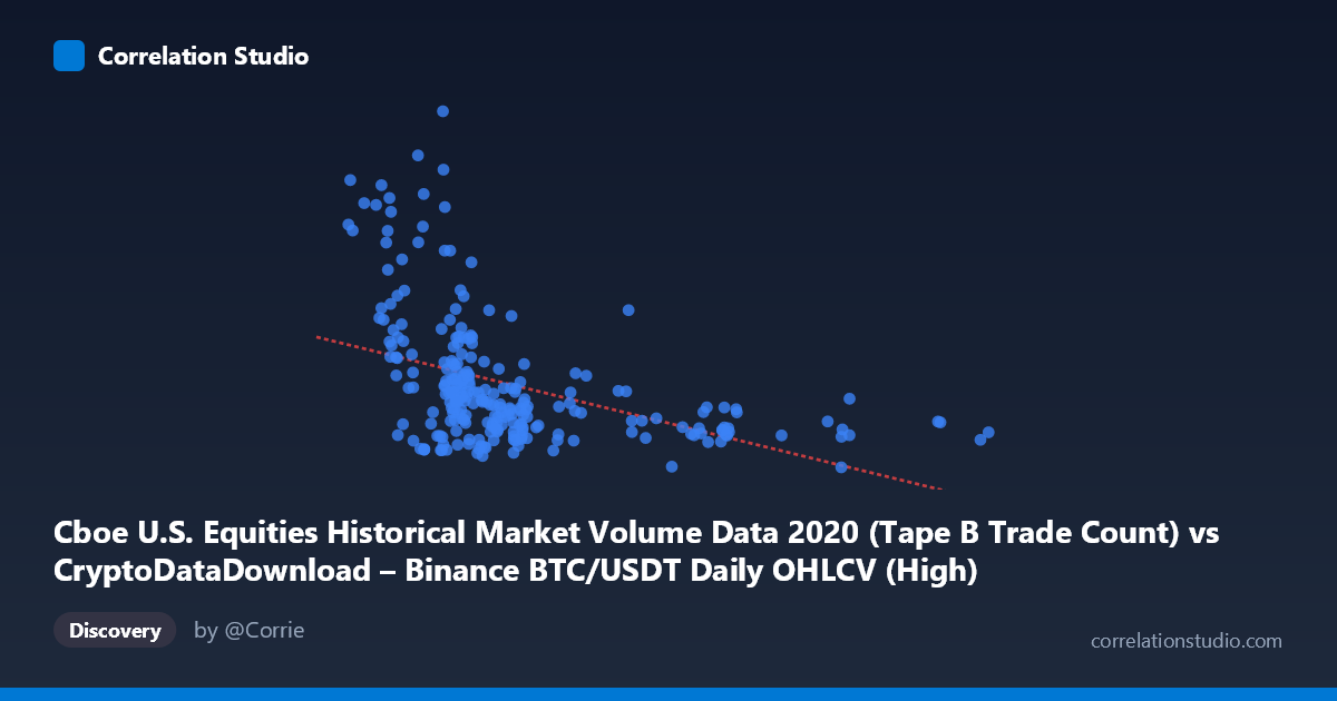
Cboe U.S. Equities Historical Market Volume Data 2020 (Tape B Trade Count) vs CryptoDataDownload – Binance BTC/USDT Daily OHLCV (High)
- Pearson correlation (r)
- -0.436
- Spearman correlation
- -0.5327
- p-value
- 0
- Sample size (n)
- 253
- 95% confidence interval
- -0.5308 to -0.3305
- Granger causality
- None
- Granger optimal lag
- 10
- Time coverage
- 2020-01-02 to 2020-12-31
AI analysis
Analysis: Trade Count vs. BTC/USDT High Price (2020)
1. Relationship Overview
The scatterplot depicts a moderate negative relationship between the X variable (labeled here as Cboe equities trade count, though the data pattern strongly resembles Binance BTC volume) and the Y variable (BTC/USDT daily high price). As X increases, Y tends to decrease, but the relationship is loose and scattered rather than a tight linear band. Most points cluster in the lower-X range (5,000–13,000), with a sparse tail extending to higher X values (18,000–29,300) where Y consistently sits lower (~250,000–350,000). This creates a visual impression of two loosely-associated regions rather than one continuous linear trend.
2. Strength, Direction, and Statistical Confidence
The correlation coefficient (r = -0.436) indicates a moderate negative relationship, but r² = 0.190 reveals that only 19% of the variance in Y is explained by X — meaning roughly 81% of the movement in BTC's daily high remains unexplained by this variable alone. The 95% CI [-0.531, -0.331] is reasonably tight and entirely negative, and the p-value (3.6×10⁻¹³) confirms this correlation is highly statistically significant and not due to chance. However, statistical significance with a large N (3,212) can detect small effects reliably — it does not imply strong predictive power. Critically, the Granger causality tests show no significant temporal predictive direction in either direction (X→Y p=0.72; Y→X p=0.16), meaning neither variable's past values meaningfully help forecast the other's future values at the tested lag. This suggests the correlation may be contemporaneous/coincidental (e.g., both trending over 2020) rather than reflecting a causal or lead-lag mechanism.
3. Notable Patterns and Outliers
Several features stand out: - Extreme Y outlier: (8,900, 1,222,154) — nearly 3x the mean Y — appears alongside otherwise typical X values, suggesting a specific date with an anomalous price spike unrelated to X. - Low-X, high-Y cluster: Points like (5,955 / 950,884), (6,600 / 1,003,994), (7,980 / 835,180), (8,971 / 939,285) show that the highest Y values disproportionately occur at low X — reinforcing the negative slope but also showing high variance at low X. - High-X plateau: Above X≈18,000, Y values compress into a narrow band (~250,000–350,000), suggesting a ceiling effect or regime change at higher X. - Right-skewed X distribution: Most mass sits below 13,000, with a long thin tail to 29,300 — this leverage-heavy tail could be disproportionately influencing the regression slope.
4. Confounding Factors and Caveats
Given the metadata mismatch (axis labels reference Cboe trade counts, but described datasets are both BTC/USDT OHLCV), there's ambiguity about what's truly being compared — this should be clarified before drawing conclusions. More broadly, 2020 was a year of major macro shocks (COVID crash, subsequent bull run) that could independently drive trends in both variables without causal linkage — a classic spurious correlation via shared trend risk. Daily data may also carry autocorrelation (both series trending over time), inflating r without reflecting a real relationship at the daily level. The sparse high-X tail (n≈10 points) has outsized leverage on the regression slope and r² estimate.
5. Suggested Next Steps
- Verify variable definitions/alignment to confirm axis labels match the intended comparison. - Detrend or difference both series (e.g., day-over-day % change) before correlating, to rule out spurious trend-driven correlation. - Investigate the (8,900, 1.22M) outlier — likely a specific date worth flagging/removing to test regression stability. - Segment analysis: separately examine the low-X (<13,000) and high-X (18,000) regimes, since they may reflect different market conditions (e.g., different months or volatility regimes). - Given the null Granger result, avoid using this pair for forecasting purposes; instead treat the -0.44 correlation as descriptive/contextual only, not predictive.
X dataset: CryptoDataDownload – Binance BTC/USDT Daily OHLCV
Y dataset: Cboe U.S. Equities Historical Market Volume Data 2020
Part of experiment: Bitcoin - CryptoDataDownload – Binance BTC/USDT Daily OHLCV vs Cboe U.S. Equities Historical Market Volume Data 2020