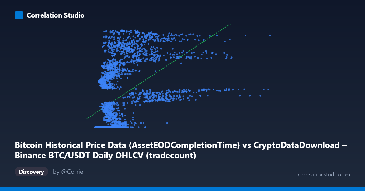
Bitcoin Historical Price Data (AssetEODCompletionTime) vs CryptoDataDownload – Binance BTC/USDT Daily OHLCV (tradecount)
- Pearson correlation (r)
- 0.5264
- Spearman correlation
- 0.7892
- p-value
- 0
- Sample size (n)
- 3191
- 95% confidence interval
- 0.5009 to 0.5511
- Granger causality
- None
- Granger optimal lag
- 10
AI analysis
Analysis: BTC/USDT Timestamp vs. Tradecount Relationship
Note on variable interpretation: The X-axis values appear to be a mislabeled or transformed version of the timestamp/completion time field (values ranging from ~2,000 to ~15.3 million don't correspond to typical Unix timestamps), and Y represents tradecount. Given the strict monotonic relationship between time and the row index in a daily dataset, X is likely functioning as a proxy for chronological sequence. This context is essential for interpreting the pattern below.
1. What the Visualization Reveals
The scatterplot shows a clear non-linear, saturating pattern rather than a simple linear trend. At low X values, Y clusters tightly near a floor around 1,614,337,000–1,614,338,000 — visible in numerous sample points (X < ~1,000,000) that all map to nearly identical Y values. As X increases, Y rises steeply and then continues climbing toward the upper range (~1.78 billion), suggesting an early "flat" regime followed by rapid growth — consistent with a logarithmic, square-root, or piecewise/step-function shape rather than a straight line.
2. Strength, Direction, and Uncertainty
The linear Pearson correlation (r = 0.526, r² = 0.277) indicates a moderate positive relationship, but only ~28% of the variance in Y is explained by a linear fit in X. The 95% CI [0.501, 0.551] is narrow and the p-value ≈ 0 confirms this correlation is statistically robust and not due to chance, given the large sample (n = 3,191). However, statistical significance here reflects sample size more than practical linear fit quality — 72% of Y's variance remains unexplained linearly. The note that Spearman ρ exceeds Pearson r reinforces that a monotonic but curved relationship fits better than a straight line. Critically, Granger causality tests show no significant predictive direction in either direction (X→Y: p=0.447; Y→X: p=0.657), meaning neither variable's history helps forecast the other in a time-series sense — undermining any causal or forecasting narrative between them.
3. Notable Patterns and Outliers
The dominant feature is the flat "floor" cluster at Y ≈ 1,614,337,000–1,614,338,000 spanning a wide range of X (from near 0 up to ~2 million), followed by a steep ascending arm as X grows further. This looks like a regime change or threshold effect — possibly an early period where the Y-metric (tradecount) was capped, not yet tracked, or the X variable resets/restarts multiple times (e.g., multiple time series concatenated). Several points (e.g., X≈2,388,458 → Y≈1,777,690,773 and X≈4,189,133 → Y≈1,775,211,617) show high Y at moderate X, while other similar-X points (X≈2,092,561 → Y≈1,642,831,104) sit much lower — indicating substantial scatter/non-monotonicity in the mid-range, not a clean function.
4. Confounding Factors and Caveats
The likely mismatch between the stated "timestamp" axis and its actual numeric range (2,153 to ~15.3M, inconsistent with Unix time) suggests X may actually be a derived index, row count, or transformed value — this ambiguity is a major caveat. Additionally, both variables are individually trending over time (Y stdev is huge relative to its range, X spans several orders of magnitude), so apparent correlation may partly be a spurious artifact of two non-stationary series both drifting over the sample period — a classic time-series confounding issue, which the null Granger result actually supports (no genuine lead-lag relationship, just shared trend/drift).
5. Actionable Insights
1. Clarify the X-axis definition — verify whether it's truly a timestamp, an index, or a transformed feature; this fundamentally changes interpretation. 2. Fit non-linear models (log, sqrt, piecewise, or spline regression) given the Spearman/Pearson divergence and visible saturation curve — likely to substantially improve fit over the current 27.7% R². 2a. Segment the data into the flat-floor regime and the ascending regime and analyze each separately, as they may reflect distinct underlying processes (e.g., early exchange history vs. later high-volume trading). 3. Detrend both series (e.g., differencing) before further correlation/causality testing to rule out spurious correlation from shared non-stationarity, since raw-level Granger tests can be unreliable without stationarity checks.
X dataset: CryptoDataDownload – Binance BTC/USDT Daily OHLCV
Y dataset: Bitcoin Historical Price Data
Part of experiment: Bitcoin - CryptoDataDownload – Binance BTC/USDT Daily OHLCV vs Bitcoin Historical Price Data